Los Angeles

Ground Calibration of an Orbiting Spacecraft Radar Transmitter

A thesis submitted in partial satisfaction of the requirements for the degree Master of Science in Electrical Engineering

by

Jon Trent Adams

1999

The thesis of Jon Trent Adams is approved.

University of California, Los Angeles

1999

Table of Contents

1 Overview *

2 A Brief Primer on the QuikSCAT Spacecraft / Mission *

3 CGS Detailed Design *

4 Analyses *

5 Conclusion *

6 Appendix *

7 References *

Figure 6-1 CGS Track Calculator User Interface 109

Table 1-1 Primary CGS Specifications *

I wish to acknowledge the following people:

At UCLA, my advisor Yahya Rahmat-Samii, for his patience, thoroughness and suggestions;

At the Jet Propulsion Laboratory, the Scatterometer Programs Manager James Graf, Section Manager Alaudin Bhanji, deputy Section Manager Richard "Bud" Lovick, and fellow employees for their interest, support, enthusiasm and patience.

Abstract of the Thesis

Ground Calibration of an Orbiting Spacecraft Radar Transmitter

by

Jon Trent Adams

Master of Science in Electrical Engineering

University of California, Los Angeles 1999

Professor Yahya Rahmat-Samii, Chair

This thesis describes a novel Calibration Ground Station (CGS) for the SeaWinds Scatterometer instrument which launches on-board the QuikSCAT spacecraft in mid-1999. The mission of this CGS is to observe the overflight of the spacecraft and accurately measure important SeaWinds instrument characteristics such as transmitter output power, pulse shape, pulse period, and Doppler offset, among other parameters. There are significant challenges in doing this successfully due to the periodic rotation of the spacecraft antenna. The required accuracy of the measurement forces an integrated approach to a novel system design to accommodate, remove or reduce amplitude error.

1. Overview
1. Introduction

The QuikSCAT Calibration Ground Station (CGS) is a dedicated 13,402 megahertz (MHz) Ku-Band receiving station which accurately measures the output characteristics of the orbiting SeaWinds scatterometer radar. The CGS is located at the NASA-Johnson Space Center White Sands Test Facility at Las Cruces, New Mexico. It is an autonomous facility with the resultant data product promptly available via the Internet.

The QuikSCAT spacecraft (s/c) carries the SeaWinds scatterometer. The scatterometer is a radar designed to illuminate the ocean's surface and record the resultant backscatter, hence the term "scatterometer". The radar signal from the spacecraft is centered on 13,402 MHz. It is a narrow-band chirped pulsed signal with a rectangular amplitude envelope. The backscatter signal is heavily post-processed and used to estimate the surface wind speeds to better than 1 meter per second over the global ice-free ocean.

The nature of the orbit geometry, the wobble of the spacecraft platform, and the rotation of the spacecraft radar antenna add an additional level of complexity to the observation. The platform, QuikSCAT, resides in a low Earth orbit with a orbital period of 101 minutes. The orbit ascending node, orbital altitude and inclination causes observing times to occur approximately twice a day, once at sunrise and once at sunset. The scatterometer antenna is a pencil-beam with dual offset feeds and rotates on a nadir-aligned axis at 18 revolutions per minute (rpm). The "inner" beam has an E-field that is oriented vertically with respect to the Earth's surface and is inclined at an angle 40º from the spacecraft nadir. The second beam is horizontally polarized and is inclined at an angle of 46º from the spacecraft nadir. The pair of antenna beams paint on the Earth's surface a never-ending dual spiral path that spans approximately 1800 km in width.

Amplitude Measurement Absolute Accuracy	± 0.25 dB 3s
Amplitude Measurement Relative Accuracy	± 0.1 dB 3s over any 4-day period
Time Measurement Absolute Accuracy	± 5.0 m s against UTC
Time Measurement Relative Accuracy	± 1.0 m s
Frequency Measurement Accuracy	± 10 Hz
Data Product Ready Time	< 30 minutes after end of pass

Table 1-1 Primary CGS Specifications

 

The goal is to create a station design that is simple, stable and most importantly provides repeatable measurements to the specifications described in Table 1-1. In order to achieve amplitude stability, the design attempts to reduce as much as possible the complexity of the analog portion of the station. Once the analog signal is digitized, it is immune to change.

The station is not only a precision receiver but a sensitive radiometer. The radiometer function provides the ability to calibrate the receiver by using both sky and local targets of known temperature and stability. The majority of the accuracy is due not only to stable equipment but more importantly to data integrated over extended observation periods. Receiver technology allows for relative stability to hundredths of a dB and absolute measurement accuracy of 0.1 dB, due mostly to the calibration standards available.

The CGS receiver uses a 20 dB-directivity, corrugated circular-aperture, circularly polarized horn on a computer-steered pedestal. This antenna was purposely chosen to be relatively immune to minor pointing errors and polarization misalignments between the spacecraft and the CGS.

The receiver downconverts the received signal in two steps. Two stages were chosen to minimize the complexity of the analog circuitry and at the same time keep the filtering requirements simple.

The 2^nd IF is at 35 MHz and is digitized into 12-bit words at a 41 megasample per second rate. Since the actual signal bandwidth is slightly more than 1 MHz, this represents a huge oversampling and produces an output that is suitable for decimation so long as the sampling is sufficiently well-behaved.

The resultant data stream is decimated by 8 and streamed into a 1 gigabyte (GB) First In, First Out (FIFO) memory space. Once the spacecraft pass is concluded, the CGS then spools the collected data onto a hard drive for permanent storage.

At this point the digital signal processing takes place. Since there is a priori knowledge about the actual spacecraft transmitter pulse width and Pulse Repetition Frequency (PRF), software performs a correlation scan through the data to find the pulse stream using this pre-knowledge. The software then precisely locates the beginning and end of each pulse, calculates the total power within the pulse, and records this information. Counting zero crossings during the pulse, it can make an estimate of the average transmitter frequency.

A Fast Fourier Transform (FFT) engine then processes the data after digitally de-chirping the signal using estimates of the appropriate de-chirp waveform. The power received will be resolved into a limited number of frequency bins and thus an accurate estimate of pulse center frequency can be generated. The FFT bins can then be summed to determine in a different manner the total pulse power. In addition, estimates of pulse chirp linearity may be reduced from this data. There are other data products extractable from this data stream also.

Once the data has been processed, the software generates an output data file containing these primary products along with stationkeeping data such as local weather, station calibration data and other information potentially important to the quality of the observation. The software then stores this file, along with the raw data set, on an FTP and HTTP server at the site so that the CGS products are available to the outside user community.

2. CGS Statement of Purpose

The QuikSCAT Calibration Ground Station shall perform regular, repeatable and accurate measurement of the QuikSCAT scatterometer transmitter Equivalent Isotropic Radiated Power (EIRP), timing and frequency, and shall make these data products available over the Internet on a timely basis.

3. Design Philosophy

The specifications levied on the CGS are challenging. There are many tradeoffs in creating a design that is robust enough to operate autonomously but at the same time make stable and repeatable observations to the accuracy required. These include the reduction of the quantity of components in the analog portion of the receiver, careful and adequate monitoring of the CGS environment, both inside and outside the facility. It is critical to understand and monitor of the atmosphere in the line of sight between the spacecraft and the CGS. The CGS antenna pointing system needs to be reliable and accurate without becoming overly complicated and expensive.

The first consideration in the design of the CGS is to choose an antenna that contributes little or no perceptible error in the desired measurement. Since the target is moving in the sky, an omni-directional antenna that is fixed in orientation comes to mind as a low-risk solution. However, the capture area of the omni is very small, and it sees an entire hemisphere so if there are sources of multipath or other emitters out there it may be very susceptible to them.

A high-gain antenna greatly reduces the multipath problem, but greatly increases the pointing requirements to maintain accuracy. The s/c position in the local sky is predicted via an orbit propagation program. The accuracy of this prediction is entirely dependent on the quality of the orbital elements or the interpolation of orbital positions used for the prediction. In the case of this particular s/c, the actual position error can be as much as 5 km Circular Error Probability (CEP) from the calculated position. This corresponds to an angular error of as much as 0.2º from the predicted position. Also, the mechanical pointing error due to the antenna pedestal may be on the order of 0.1º and nearly undetectable since it is difficult to accurately calibrate the pedestal over the entire hemisphere.

Thus, the best choice quickly becomes a medium-gain antenna, with a broad, flat beam nose, so that even with all the potential pointing and predict errors the error due to the s/c not being in the dead-center of the beam is negligible.

The receiver design should be as simple as practical. The less the total count of analog components in the receiving chain, generally the more stable in amplitude the receiver's characteristics will be.

But amplitude stability is only half the answer; gain knowledge is the other half. A stable and well-calibrated noise source must be available to provide the ability to measure and estimate regularly absolute and relative gain and gain stability.

Frequency stability of the receiver is critical due to the requirements to estimate transmitter frequency. While ultra-stable, stand-alone oscillators are available, they are expensive and carry with them the requirement to maintain knowledge of their exact frequency and/or correct them over time. It is preferable to use an in-situ system that someone else maintains, when possible. Since the facility at which the CGS is housed has no ready-made distribution of ultra-stable reference frequency, use of the Global Positioning System (GPS) for ultra-stable frequency and timing reference proves to be a simple and very inexpensive solution to the dilemma.

The final point of design simplification for the purposes of accuracy comes at drawing the dividing line between the analog and digital portions of the CGS. As mentioned before, the point at which the incoming signal is digitized is the point at which the received signal data becomes immutable. It is advantageous to do this as close to the front end as practical.

High-quality (stable, high-resolution, low aperture jitter, well-characterized, etc.) Analog-to-Digital Converters (ADCs) are generally available and relatively inexpensive. The bandwidth of the information that must be recorded is only a few megahertz. As long as the sample jitter is very low, the signal can be sampled at a high RF frequency and digitally decimated to produce a low-data-rate bit stream that will not overwhelm the capture and storage system.

The storage system required must be able to manage the high instantaneous data bandwidth (10 MB/sec) over the duration of an entire pass (consisting of up to 4 points of 10 seconds each plus all the calibration data), keeping very accurate track of the exact time of capture of each bit. To this end it appears most practical to use a large solid-state memory buffer to capture the entire pass (up to about 500 MB of data) then spool that to a hard drive for storage and subsequent processing.

---

 

2. A Brief Primer on the QuikSCAT Spacecraft / Mission

1. The QuikSCAT Spacecraft

The QuikSCAT spacecraft is carried aboard a Titan II launch vehicle and is scheduled for launch in the spring of 1999. Figure 2-1 is an artist's rendition of the QuikSCAT spacecraft in Earth orbit. Figure 2-2 is a conceptual block diagram that shows the spacecraft and the SeaWinds radar scatterometer antenna attached to its nadir surface.



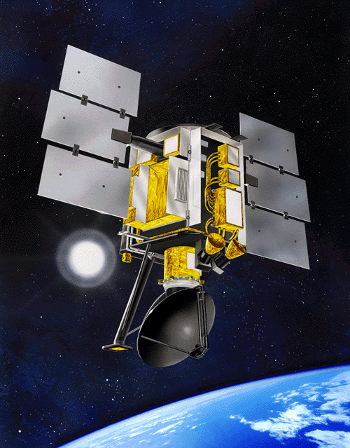
Figure 2-1 The QuikSCAT Spacecraft

The SeaWinds scatterometer is installed on the QuikSCAT spacecraft and is in fact the only science instrument aboard. The SeaWinds instrument is a specialized microwave radar that measures oceanic near-surface wind speed. The SeaWinds on QuikSCAT mission is a "quick recovery" mission to fill the gap created by the loss of data from the NASA Scatterometer (NSCAT), which occurred when the Japanese spacecraft it was carried on lost its solar panel in June 1997. QuikSCAT, scheduled for launch from California's Vandenberg Air Force Base aboard a Titan II vehicle in spring 1999, will continue the important mission begun by NSCAT in September 1996 to collect ocean wind data sets.

SeaWinds uses a rotating dish antenna with two spot beams that sweep in a circular pattern. The antenna radiates microwave pulses at a frequency of 13.4 gigahertz (GHz), each pulse illuminating 1500 km² areas of the Earth's surface. The instrument collects data over ocean, land, and ice in a continuous, 1,800-kilometer-wide band, making over 22 million measurements and covering 90% of Earth's surface in one day.

QuikSCAT launches into a sun-synchronous, 803-kilometer, circular orbit with a local equator crossing time at the ascending node of 6:00 A.M. +/- 30 minutes. Data acquisition is facilitated by NASA Wallops Flight Facility which manages, implements, and operates the NASA tracking stations at Poker Flats Station (Alaska), Wallops Flight Facility (Virginia), Svalbard Station (Norway), and McMurdo Station (Antarctica). The distribution of the science data to NOAA-Suitland for operational uses, and to JPL for science processing, is via electronic transfer. Wind data is available for weather forecasters within three hours of observation. Japan's National Space Development Agency (NASDA) also supports the mission by providing science and instrument adjustment support, as well as backup for tracking stations.

The Jet Propulsion Laboratory, operated by the California Institute of Technology, manages the SeaWinds on QuikSCAT project for NASA's Earth Science Enterprise.

2. SeaWinds on QuikSCAT



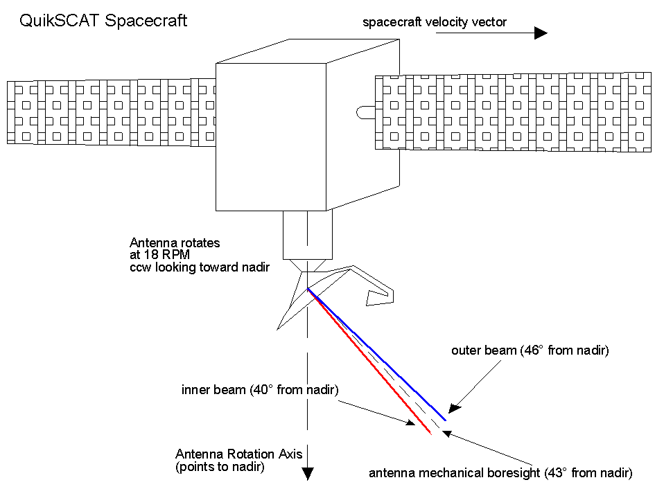
Figure 2-2 Generalized Diagram of SeaWinds on QuikSCAT

 

Onboard the spacecraft is the SeaWinds radar scatterometer instrument (Figure 2-2). The SeaWinds antenna rotates at 18rpm, or 108º of arc per second, on a nadir-pointing axis, and the antenna mechanical boresight lies at an angle of 43º from the nadir. The feed structure for the antenna has two orthogonally polarized horns that form pencil beams each pointing 3° off-boresight but in opposite directions. The two beams thus formed are 40° and 46° from nadir. The inner beam has a nominal 1.6° half-power beamwidth while the outer beam has a 1.4° beamwidth. Part of the reason for the difference is that the outer beam strikes the Earth's surface at greater range, and so there is greater path loss. The narrower beam helps to make up for this with about 1dB more gain, providing about 2dB extra gain total on the round-trip. The other, equally important reason, is that the mission requires a similar resolution of measurement from each beam, and so the outer beam's smaller arc diameter makes for a spatially-similar footprint.

3. Orbital Geometry

Figure 2-3 shows the QuikSCAT s/c orbit orientation to Earth and the Sun. The orbit is slightly retrograde (orbits against the rotation of the Earth) and sun-synchronous. Orbits are generally specified with six parameters: orbital altitude above the equator; the eccentricity of the orbit (remember that orbits are ellipses - thus the eccentricity is the ratio of focus-to-center distance divided by the semi-major axis); inclination of the orbital plane to the equatorial plane; longitude of ascending node specifies the terrestrial longitude at which the sub-satellite point of the orbiting crosses from the southern to the northern hemisphere at the beginning of its orbit cycle; argument of perigee specifies the tilt of the semi-minor axis; and the mean anomaly is an angle that increases uniformly with time, starting at perigee. The nominal orbital elements for this orbit are summarized in Table 2-1.

 

 

Parameter	Value
Orbital Altitude (@ equator)	803.0km
Eccentricity	0.0015
Inclination	98.6º (retrograde)
Longitude of Ascending Node	90.0º
Argument of Perigee	90.0º
Mean Anomaly at 0h GMT	0

Table 2-1 Nominal Orbital Elements

 



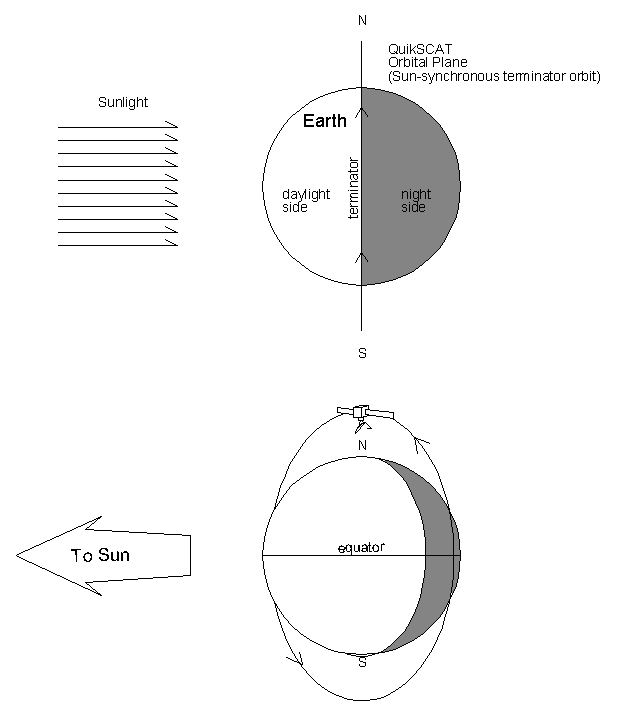
Figure 2-3 Generalized Orbital Orientation

 

The QuikSCAT orbit is nearly circular, with an orbital period of 6060 seconds (101 minutes). Since it is highly inclined, it actually rotates against the direction of Earth's rotation and thus appears to remain fixed in a plane approximately perpendicular to the Sun-Earth line. This orbit is called a "terminator" orbit since the majority of the time the spacecraft is straddling the boundary between night and day as diagrammed in Figure 2-3.

What this also means is that the passes over the CGS, located at approximately 30º north latitude, will be from south-southeast to north-northwest and from north-northeast to south-southwest. This is important to know since it will constrain the possible azimuthal look angles for the CGS to track the spacecraft.



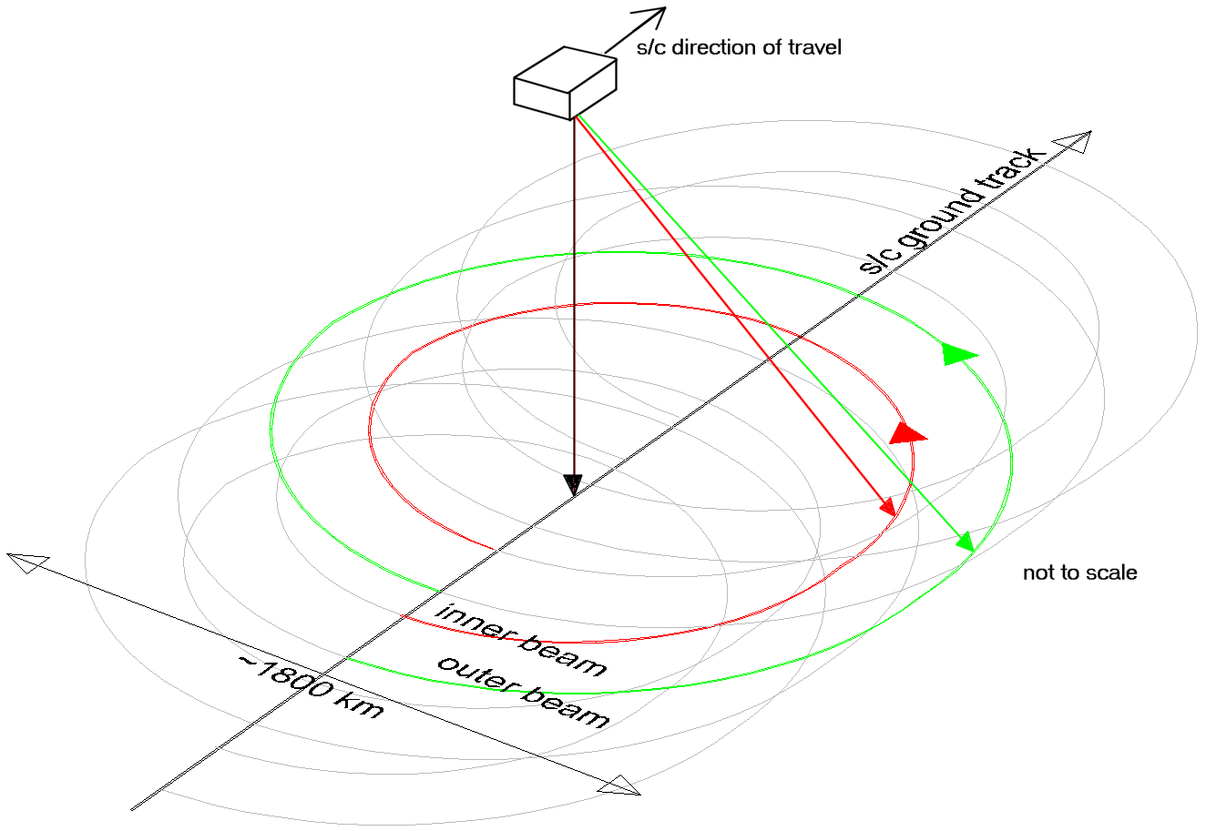
Figure 2-4 Generalized Ground Track of Spacecraft Antenna Beams

Figure 2-4 is a generalized view of the spacecraft antenna beam pattern on the ground. The inner beam describes a helix 40º offset from nadir and of radius 1400 km, while the outer beam describes the outer helix 46º away from the nadir. The width of the swath painted by the outer beam is approximately 1800km.

The orbit is set to repeat its pattern on a four-day basis. This means that four days after the spacecraft flies over a given point on the Earth it shall pass over that point again, repeating the orbit exactly. (The spacecraft orbit will be adjusted as necessary to maintain the exact repeat structure.) This is valuable to know since it fully constrains the orbit and thus the potential pass angles as observed at the CGS. In fact, due to the orbital parameters, the CGS will have the opportunity generally to observe between 4 and 7 optimal passes over a 4-day period and the pointing angles needed to capture these passes will always be the same.



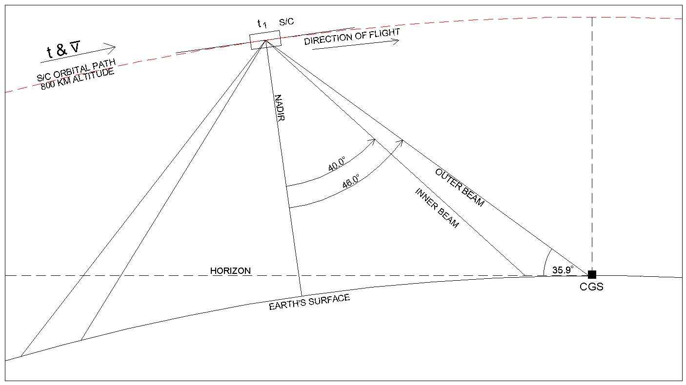
Figure 2-5 Spacecraft / CGS Antenna Beam Incidence Angles (outer)

 

Figure 2-5 is a scale, elevation view of the orbital geometry as the outer beam first intersects the CGS. It is important to note that so long as the spacecraft platform wobble is well-controlled (and it should be), the outer beam always intersects the ground at an angle 35.9° above the horizon. This geometry is described in Figure 2-6 for both the inner and outer beams.



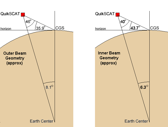
Figure 2-6 Inner and Outer Beam Geometry

 

Thus, this reduces the requirements for the CGS pointing to one elevation angle for intersecting the outer beam.



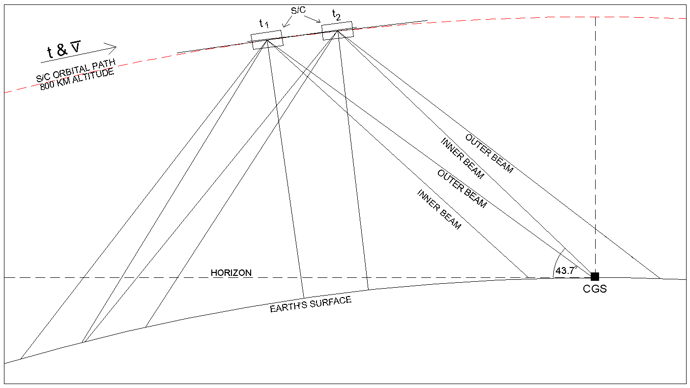
Figure 2-7 Spacecraft / CGS Antenna Beam Incidence Angles (inner)

Figure 2-7 is a scale, elevation view of the orbital geometry about 20 seconds later when the inner beam first intersects the CGS. Again, so long as there is good spacecraft attitude control, the inner beam always intersects the ground at an angle 43.7° above the horizon (See Figure 2-6). Thus, this reduces the requirements for the CGS pointing to one elevation angle for intersecting the inner beam.



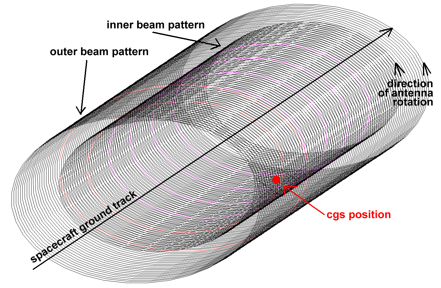
Figure 2-8 Actual Ground Track of Spacecraft Antenna Beams

 

Figure 2-8 is a "scale" model version of the simplified diagram shown in Figure 2-4. Optimal scatterometer coverage is provided for any point on the Earth that is illuminated by both the inner and outer beams during a single pass. This requires that the point on the ground be somewhere between the nadir point and the edge of the inner beam rotation. The pitch of the dual-helix is very tight due to the fast rotation of the spacecraft antenna and the relatively slow along-track spacecraft velocity of 7.4km per second. A potential "good" (see ¶2.3.1) CGS position is indicated on the figure, since from that position the CGS will be illuminated by both the inner and outer spacecraft beams.

 

1. Good and Not-so-Good Orbital Passes

Due to the repeating nature of the orbit, and the fact that the CGS is at a relatively low latitude (30º N), the longitude of the ascending node of the orbit plays a strong influence on the general quality of the passes observable from the CGS. As Figure 2-9 indicates, these passes include ones where: The CGS intercepts neither of the beams (missed pass); the CGS intercepts the outer beam but not the inner beam (minimum pass); the CGS intercepts both the inner and outer beam (good pass). It is desirable from a calibration point of view to have the spacecraft make only good passes over the CGS; in reality, though, this is impossible.



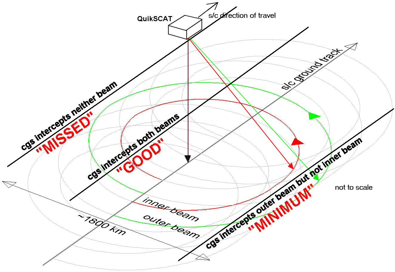
Figure 2-9 Good and Not-So-Good Passes



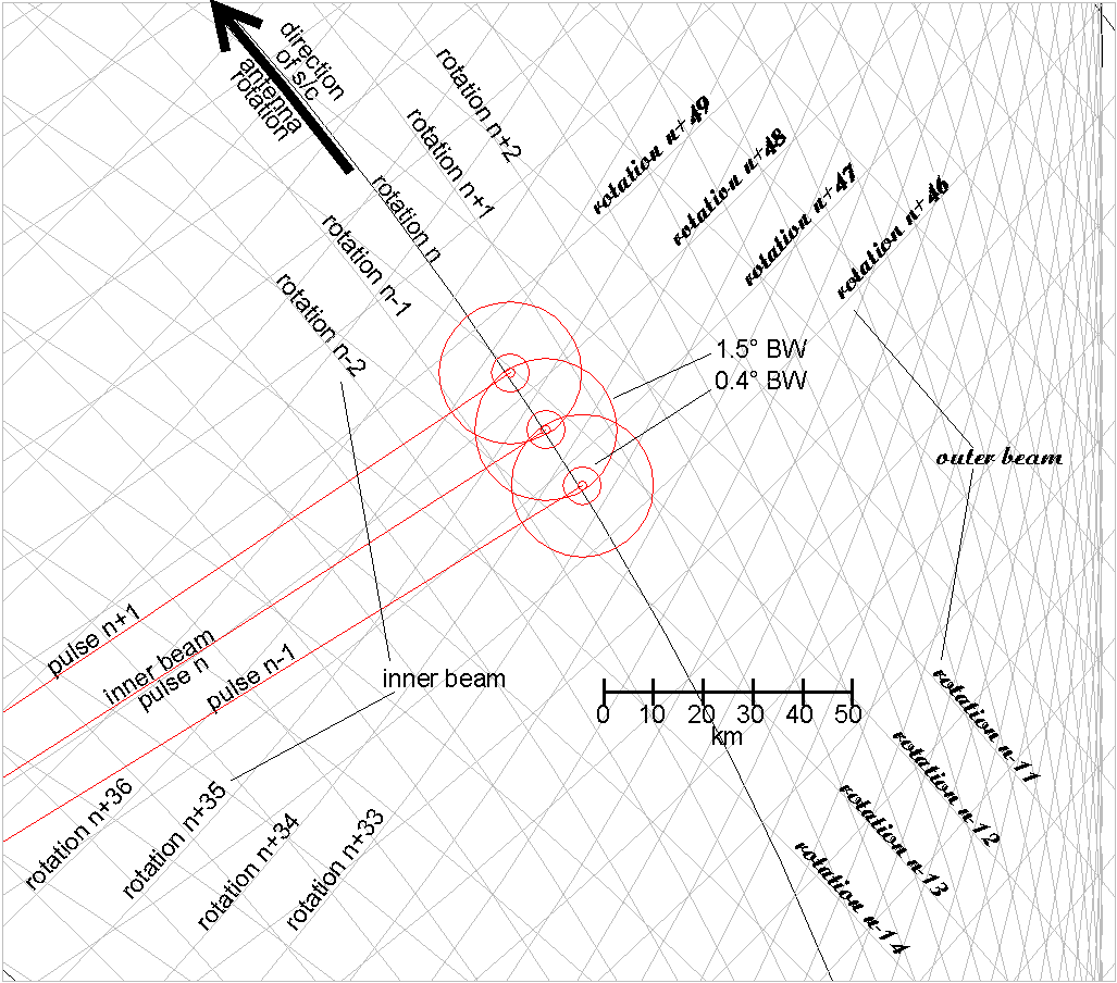
Figure 2-10 Composite View of Antenna Beam Ground Tracks during one Good Pass

 

Figure 2-10 is a section of a plot of the ground track of the two beams as they pass across a section of the Earth. In this figure, the three circle groups represent individual 1.5 ms pulses transmitted once every 5.4 ms. The spacecraft antenna rotates anti-clockwise at 108° per second, or 0.54° per PRI. The circle groups are separated by 0.54° (along-track spacecraft velocity is about 1/200^th of the rotational velocity and therefore may be ignored).

The three pulses mapped on the figure were radiated from the inner beam of the spacecraft antenna during spacecraft antenna rotation n. One antenna rotation represents 3.33 seconds of time. The ground track of both earlier and later antenna rotations are mapped as rotations n-2, n-1, and n+1, n+2. At the time of these rotations, this patch of ground is still forward of the spacecraft. About 34 antenna rotations later (100 seconds) the spacecraft antenna will illuminate the same area, except now the spacecraft will be looking aft. These rotations are indicated as n+33, through n+36.

The chart also shows the illumination of the same area by the outer beam of the spacecraft antenna. These rotations are shown in script lettering. The numbering for the outer beam rotations is relative to inner beam rotation n. Thus, the outer beam (which leads the inner beam; see Figure 2-5) swept out several rotations over this area at n-14 through n-11, and will again sweep over the area at n+46 through n+49.

During one good spacecraft pass, the CGS will have the potential to be illuminated directly 4 times by the spacecraft antenna.



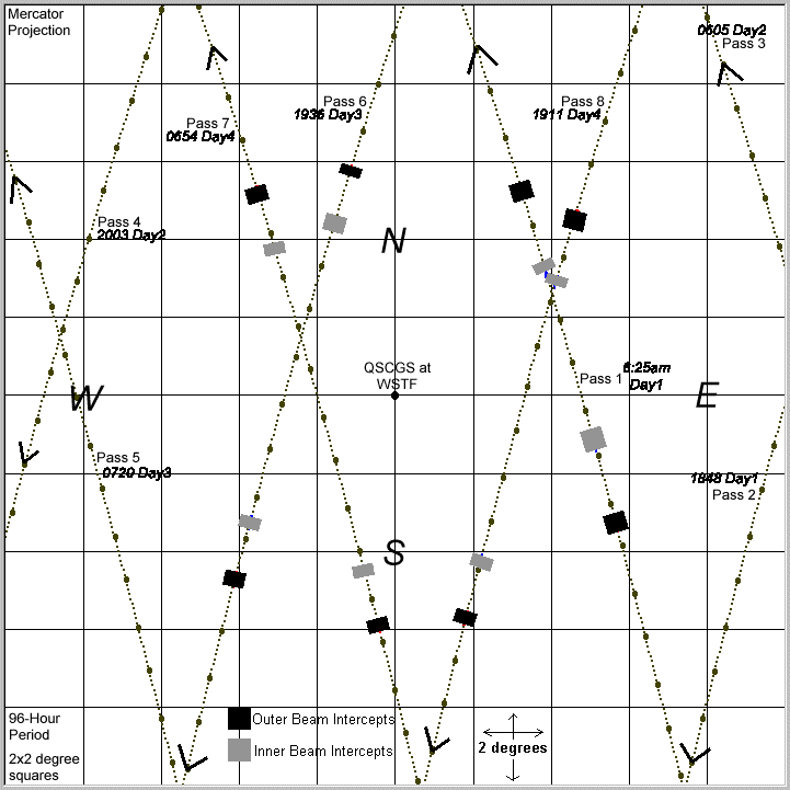
Figure 2-11 CGS 4-Day Pass Profile (Asc Node = 0 deg)

 

Spacecraft passes at the CGS are infrequent due to the orbital parameters and the latitude of the CGS. Figure 2-11 is a Mercator projection map generated by the author's CGS Track Calculator program. The passes are marked for day and time of day at pass center, and the larger dots on the path lines represent 20 seconds of time. The small dots between the larger ones are 2 second ticks. The orbit depicted is arbitrary since the longitude of ascending node parameter is undetermined at this time and causes the orbit to skew east or west. However, for this arbitrary orbit the CGS has opportunities to observe 4 good passes (passes 1, 6, 7, 8) and 4 missed passes (passes 2, 3, 4, 5) during the 4-day period.

The good passes in the diagram show the period of time in which the spacecraft inner or outer beam boresight vector is within ±1° of the CGS antenna boresight vector (i.e., when the two antennas are aimed directly at one another). The hatched areas along each pass path indicate when the inner and outer beams are each co-aligned.

For the outer beam interception, the spacecraft will be within ±1° of 35.9° above the horizon local to the CGS. For the inner beam interception, the spacecraft will be within ±1° of 43.7° above the horizon.

 

 



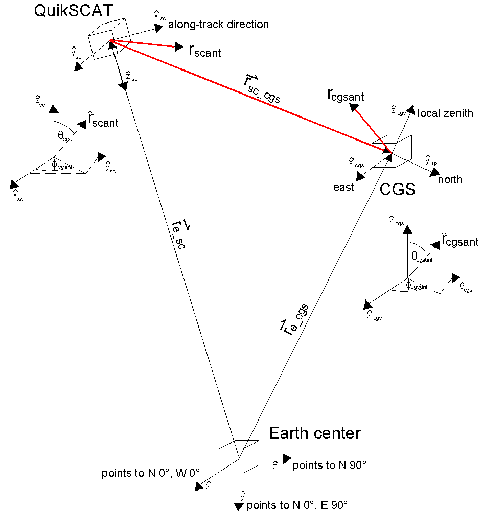
Figure -12 Three Different Coordinate Systems

 

2. Resolving the Coordinate Systems

There are three separate coordinate systems involved (Figure 2-12). In order to calculate antenna gain at both spacecraft and CGS, some vector arithmetic must be done to express the antenna coordinate systems in terms of the fixed Earth reference system. Since the position of the CGS is fixed (barring large tectonic activity), it is a simple matter to establish the CGS antenna boresight pointing unit vector.

At the CGS, latitude, longitude, elevation above mean sea level of the CGS and azimuth and elevation of the CGS antenna boresight are well known. Expressing the CGS local coordinate system in terms of the Earth reference system we get



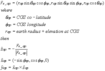
Next, we wish to describe the orientation of the CGS antenna with respect to the CGS coordinate frame.



Next, we must locate the spacecraft in the Earth's reference frame.



Once the satellite's coordinate system has been translated to the Earth's, then we locate the vector that describes the current spacecraft antenna boresight with respect to the s/c coordinate system.



Next we derive the vector that describes the path between the spacecraft and the CGS:



With this vector and the CGS normal vector, we can quickly determine using the dot product whether or not the spacecraft is above the local horizon.

If it is above the local horizon, then we need to calculate where the current antenna boresight vectors are with respect to the vector connecting the spacecraft and CGS. If we know the antenna patterns, we can use that information to look up the antenna gains at that angle off-boresight:





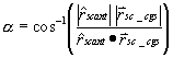
where a is the included angle between the spacecraft antenna boresight vector and the spacecraft - CGS vector; and

b is the included angle between the spacecraft antenna boresight vector and the spacecraft - CGS vector.

3. CGS Detailed Design

1. Overall System Design

The goal of the CGS design is to provide a system that has as little complexity as necessary and is essentially self-calibrating. There are obvious choices here: receiver parts-reduction and block diagram simplification; digitization of the received signal as soon as practical; use of a highly stable and well-calibrated noise source as the primary calibration reference standard. Less obvious though an equally valuable step includes temperature stabilization and/or temperature control of the entire receiver chain from antenna horn to ADC.

1. System Block Diagram

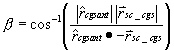
Figure 3-1 is the CGS system block diagram showing the major assemblies and signal flow. The system is divided into three major subsystems: the antenna assembly and radome; the pedestal-mounted microwave receiver; and the rack-mounted IF receiver, digital signal processor, and scheduling and control computer.



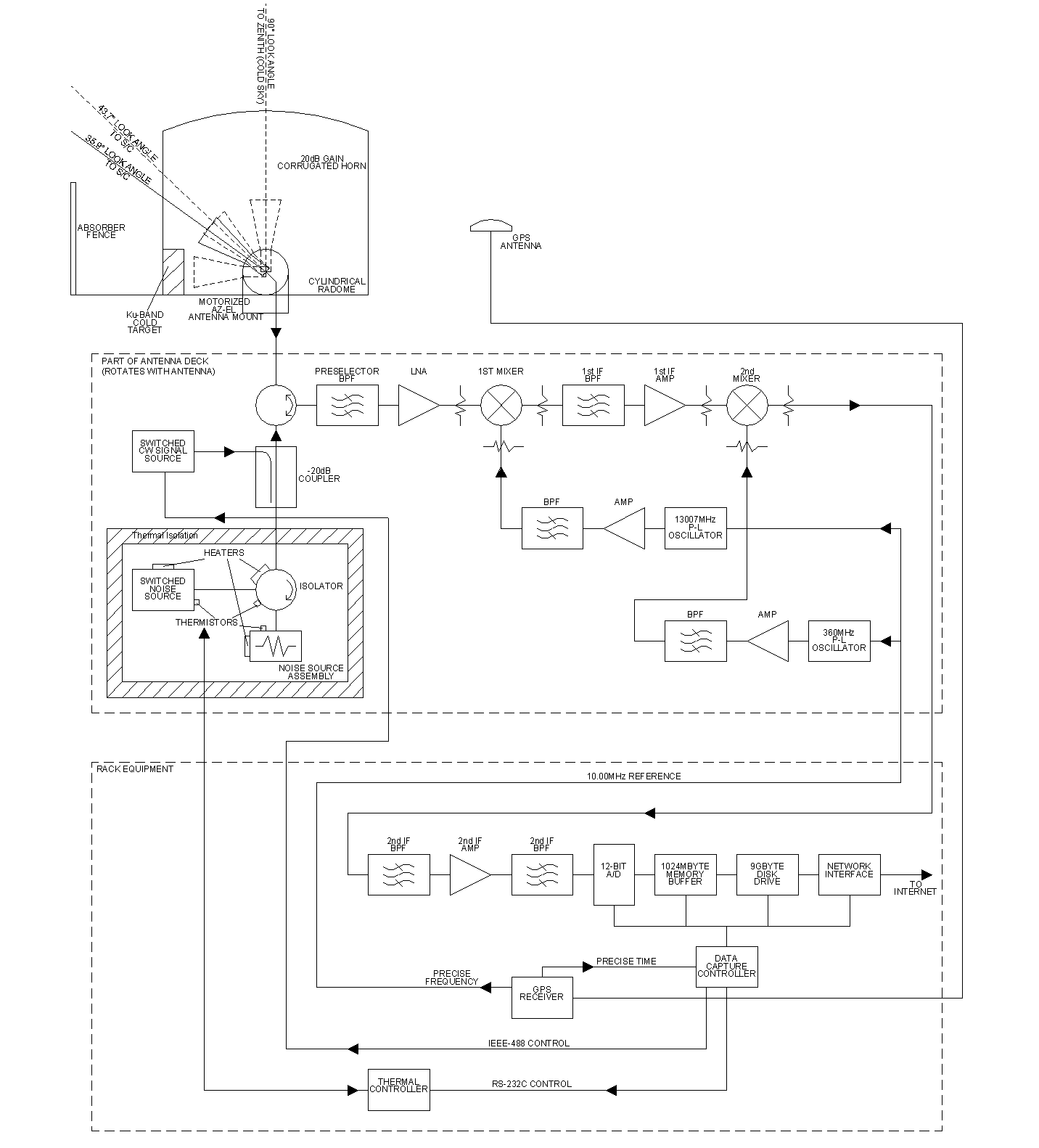
Figure -1 CGS System Block Diagram



Table -1 System Link Budget



Table -2 Error Contributions

2. Link Budget

The link budget in Table 3-1 takes into account the system from spacecraft transmitter to CGS digitizer, accounting for the RF, propagation characteristics, noise figures and receiver gains. It is meant to provide an estimate of the nominal signal-to-noise ratios in the receiver. The actual link budget table is an Excel spreadsheet that may be changed as required to keep up to date with the actual design, or to make estimates of system function if modification is required.

3. Error Contributions

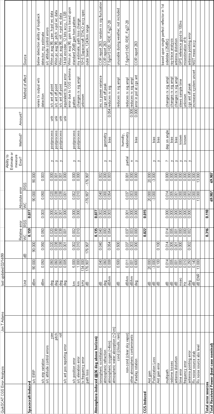
The link budget above assumes certain values from the error contribution table. The error contribution table (Table 3-2) tabulates the worst-case loss factors from the transmitter to the receiver. This includes factors such as spacecraft platform stability, loss due to atmospheric oxygen and water vapor, loss due to the CGS radome and receiver. At the left-hand side of the table, losses are collected into Spacecraft-Induced, Atmosphere-Induced, and CGS-Induced (Column 1). Column 2 indicates the types of losses. Column 5 indicates the amount of the error in the natural units of the error source (i.e., platform wobble is in degrees) while Column 6 translates the natural units of column 5 into dB. Column 5 though 10 are an attempt to aggregate the errors as being relative or absolute, and then tallying as Worst Case (WC) or Root Sum Squared (RSS). Column 11 indicates whether we believe that the error term may be estimated, measured or otherwise better known so that we can reduce the total error; Column 12 is an assumption of the technique of error reduction; Column 13 is the total error remaining after reduction. Column 14 is the method by which the error term affects the measurement; and finally Column 15 is a comment field describing the source of the error term values and other comments.

2. Spacecraft and Instrument Characteristics

1. Transmitter / Antenna / Signal Characteristics

The spacecraft radar transmitter is a simple design. It generates a rectangular pulse (constant amplitude), with a linear FM chirp (Figure 3-2). The rate of frequency change is 250 kHz/ms. The transmitter pulse period is 1.5 ms, so the total frequency change during the transmitter pulse is 375 kHz. The chirp is centered about the transmitter's nominal center frequency. The transmitter center frequency is adjusted to compensate for the expected two-way Doppler due to the radial component of the spacecraft-ground relative velocity. (I.e., if the relative velocity would produce a two-way Doppler of +480 kHz (closing on target), the transmitter center frequency is shifted -480 kHz so that the returned echo is centered within ±10 kHz of the receiver passband at 13,402.0 MHz. This pre-compensation is via a lookup table onboard the spacecraft and the individual values contained within that table are available for post-processing on the ground.

 



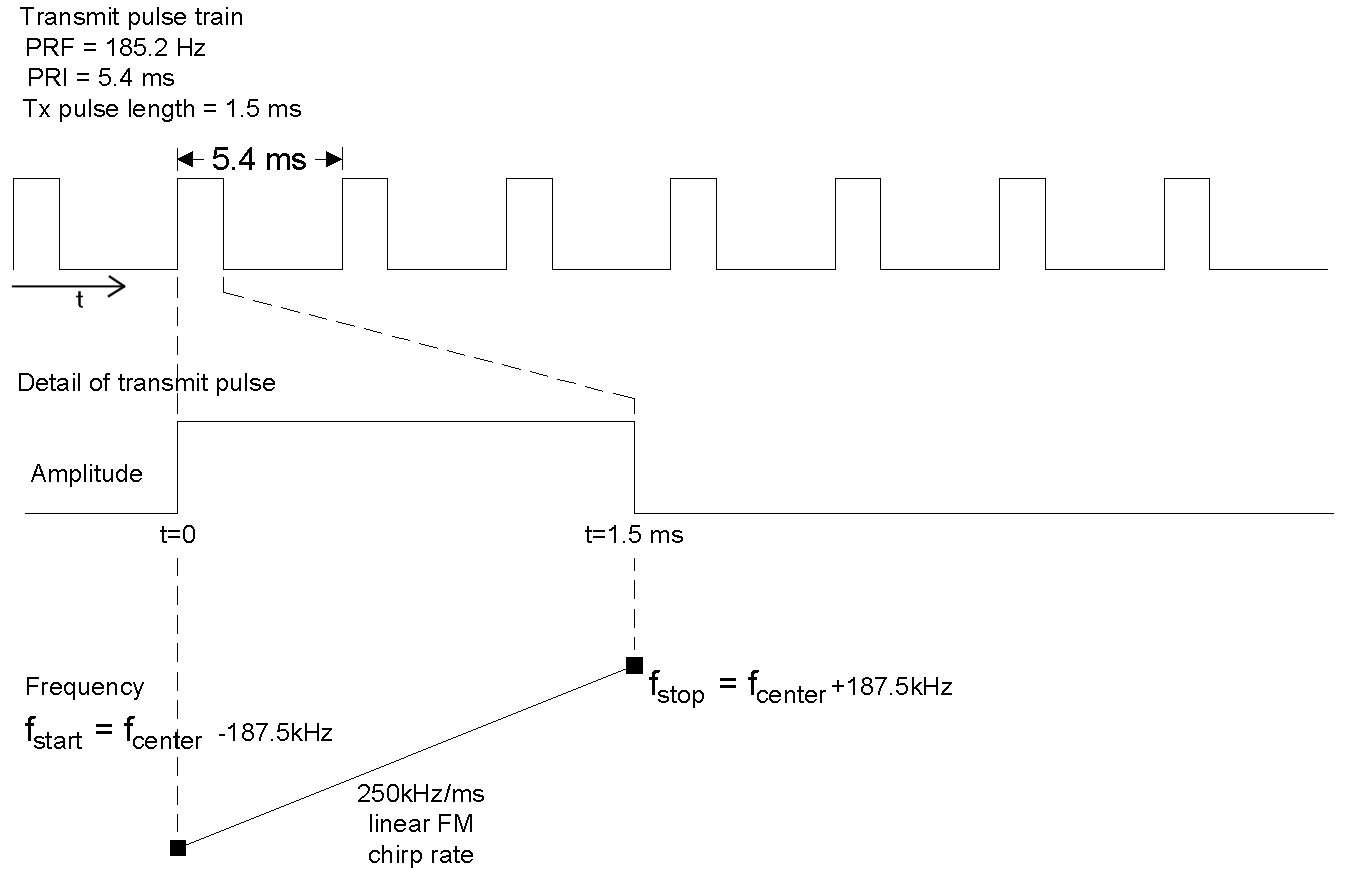
Figure -2 SeaWinds Transmitter Frequency and Timing Characteristics

 

The radar antenna is a rotating, 1 m offset-feed paraboloid with a gain of approximately 39 dB and employs two separate feedhorns to provide two separate pencil beams that are separated by 6 degrees of arc. Each is 3 degrees off the mechanical boresight of the antenna but in opposite directions. The inner beam (40° from the antenna rotation axis) is horizontally polarized. This polarization sense is with respect to the nominal impact angle with the earth (when observed on the ground, the incoming radar beam's E-field would be oriented left-right). The outer beam is positioned at 46° from the antenna rotation axis and is vertically polarized (on the ground, E-field is up-down).

The inner beam projects a pattern that has a 3 dB beamwidth of 1.6°; at the range of the target (1096 km) and the incidence angle of 44° (on the ground) this corresponds to a footprint 31 km wide by 44 km deep. The maximum antenna directivity is about 39dB. The outer beam beamwidth is 1.4°. This illuminates a footprint about 30 by 52 km in size. The differing beamwidths were chosen to minimize the difference in footprint size and to equalize the return powers from each of the footprints. The range difference of 1243 km vs. 1096 km makes for an additional path loss to the far spot of 1.1 dB, or a round-trip loss of about 2.2 dB. To compensate for this, the outer beam has a slightly higher gain. Figure 3-3 is a hybrid of the spacecraft inner beam antenna pattern (measured on a range ±20° from boresight) fitted with a Physical Optics (PO) / Physical Theory of Diffraction (PTD) model [1] of the spacecraft antenna beam directivity between 20° and 120° from the boresight. Figure 3-3 is a plot of the actual values being used in the program "CGS Track Calculator" to model the illumination cast by the s/c antenna. This is a simplification of the actual antenna pattern but since the antenna is generally symmetrical about its boresight axis, it is a reasonable assumption in order to dramatically reduce the calculations required.



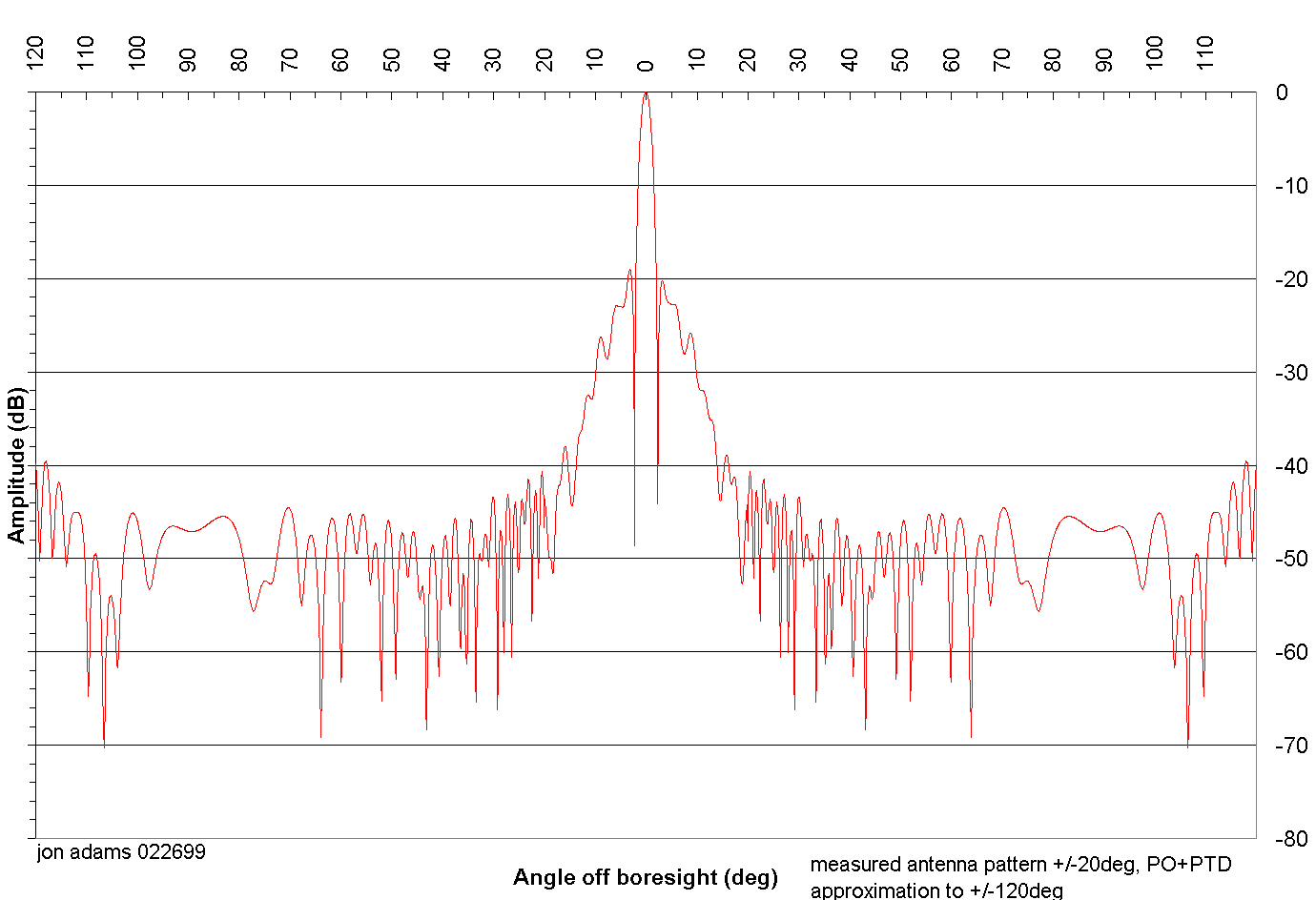
Figure -3 Spacecraft Antenna E-Plane Outer Beam Azimuth Cut (hybrid using PO+PTD and measured data)

 

The antenna rotates at approximately 18 rpm, or an angular rate of 108° per second. The radar transmitter generates 1.5 ms pulses with a PRF of 200 Hz. Thus the antenna rotates 0.54° every Pulse Repetition Interval (PRI). In addition, during the period of one transmit pulse, the antenna rotates 0.16° . On the ground at the far spot, this motion causes the footprint to move about 1700 km per second, or 8.5 km per pulse. As can be imagined, this constant antenna rotation increases the complexity of accurate power measurement on the ground.

2. Platform Attitude Control and Knowledge

The spacecraft itself plays a critical part in the overall ability to perform accurate ground-based measurements of the radar transmitter. The spacecraft attitude must remain very steady or the resultant transmitted radar beam will wobble. For the purposes of this analysis, it shall be assumed that the s/c attitude and knowledge is better than 0.01° . While challenging, this is achievable with star trackers and magnetic torquers which are installed on the QuikSCAT spacecraft.

3. Spacecraft Science and Engineering Telemetry

Finally, there is the need to correlate what is observed by the CGS with what was actually occurring on-board the spacecraft. There are two data streams returning from the s/c: the first is the science stream which consists of the actual scatterometric observations of the earth, and the second is the engineering stream which reports position, attitude, and other critical mission factors. These data are stored on the spacecraft and downloaded to an earth tracking station generally only once per 101-minute orbit, so it is impossible for the CGS to use any of these data in real time. However, it can be used in post-processing to further improve the data quality by removing s/c and instrument artifacts. In addition, it is valuable for screening the data for anomalous behavior that could skew or otherwise corrupt the data. For the purposes of this analysis though, these data will not be considered.

3. Pass Timing and Structure

The following figures provide a bird's eye view of two types of good pass and one minimum pass. Figure 3-4 shows a nominal zenith pass. Figure 3-5 shows another good pass, and one certainly more probable than the zenith pass, where the CGS still intercepts both beams twice from the spacecraft. Figure 3-6 shows another pass, this time a minimum one, where the spacecraft never rises far enough in the sky for the inner beam to illuminate the CGS.



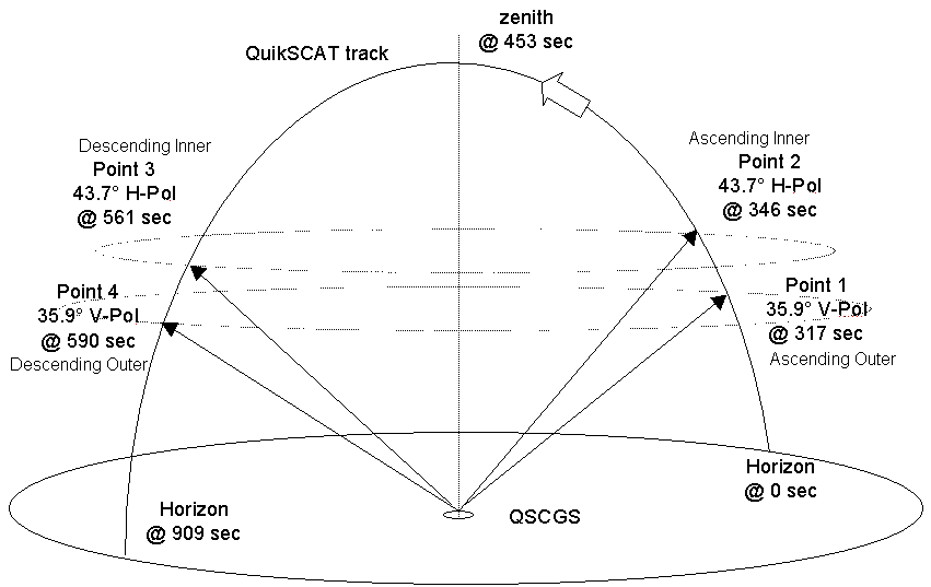
Figure -4 A Good (Zenith) Pass

 

 



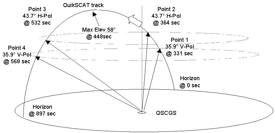
Figure -5 A Good Pass (Mid-elevation)

 



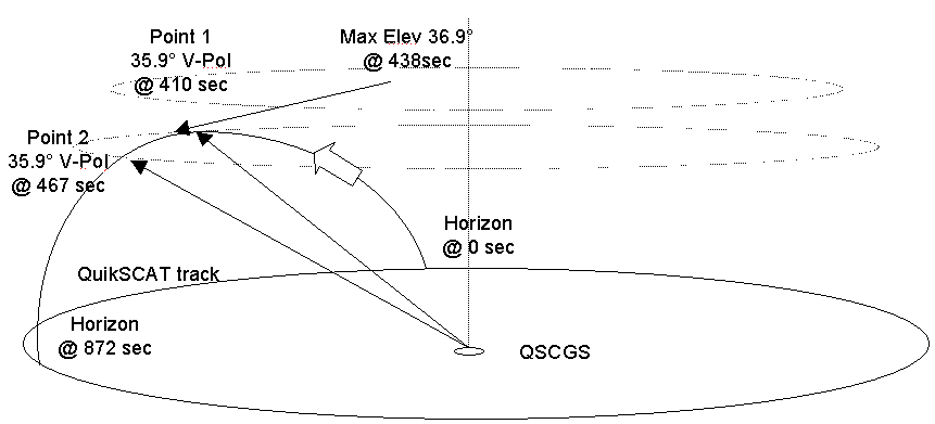
Figure -6 A Minimum Pass (Outer Beam Only)

 

The CGS, employing orbital elements received from the QuikSCAT operational group, generates an ephemeris to predict passes that can be seen from the CGS. This predict includes spacecraft local rise and set times and track across the sky in azimuth / elevation. The accuracy of the predict is better than 1 second (subject of course to the accuracy of the orbital elements).



Figure -7 General Pass Timing

 

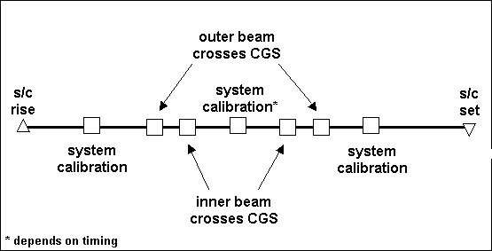
Once the pass timing is estimated, the CGS then arranges other system functions to fit the schedule. After spacecraft rise, but before the first outer beam crossing, the CGS performs an internal calibration sequence. This includes making measurements of the internal noise source and the internal room-temperature waveguide load. Once the system calibrations are finished, the CGS controller aims the antenna at the first outer beam crossing azimuth and elevation angle and waits for the spacecraft to pass through the field of view.

At a time 5 seconds before the CGS has predicted the first outer beam crossing, the CGS controller begins digitizing the receiver output. During the next 10 seconds, the CGS will digitize at a rate of about 5 megasamples per second, collecting a continuous block of about 10 MB of data. In that 10 seconds of time, the spacecraft antenna will rotate 3 times, and the signal recorded by the CGS will look something like that modeled in Figure 4-17.

Figure 3-8 shows the received pulse stream from the spacecraft. The received pulses are about 1.5 ms long, and are spaced at an interval of 5.4 ms. The CGS samples continuously whether the transmitter pulse is there or not, so not only does it capture the transmitted pulse but it also captures the periods of quiet between pulses.

Later, in post-processing, it will be these quiet periods that are accumulated to derive the radiometric noise contribution. The reason that this is done is that almost anywhere the spacecraft is in the sky surrounding the CGS, the CGS WILL hear it. Therefore, any attempt to measure noise indiscriminately (without taking into account the transmitter timing) will invariably be doomed to failure. But, since the timing is well-known and post-processing will be able to locate exactly the transmitted pulses, it is a simple thing to accumulate the noise in the inter-pulse intervals and thus come up with an accurate and very useful measure of the radiometric environment during the observation.



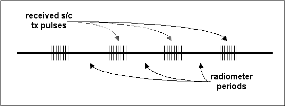
Figure -8 Timing Detail During Outer Beam / CGS Crossing (example)

 

4. Path Characteristics

1. Path Loss as a Function of Position

The s/c orbit is nominally circular, at an altitude of 803 km at the equator. The orbit period is 101 minutes, and the orbit is slightly retrograde (the s/c orbits in a direction opposite from the earth's rotation). The orbit is designed to be a terminator orbit, so that the local time at the nadir point is always either approximately sunset or sunrise. Figure 3-9 shows the variation in path length as a function of elevation when the spacecraft is above the local horizon. At the horizon, the spacecraft is at 0° elevation and is approximately 3300 km distant from the CGS; the closest the spacecraft can approach the CGS is if there is a zenith (90° ) pass when the separation distance is approximately 800 km.

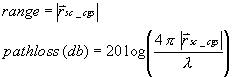
The path loss due to range is defined by the equation



This can be derived through the following: The power density in watts per square meter of an isotropic radiator is given by



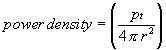
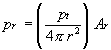
where r is the radius in meters of the sphere surrounding the isotropic radiator and p_t is the transmitter power. All power emitted by that isotropic radiator will be distributed equally on the surface of the sphere. A receiving antenna located on the surface of that sphere intercepts total power equal to the power density multiplied by the surface area of the receiving antenna as follows:



It can also be shown that a transmitting antenna of effective area A_t which concentrates its gain within a small solid angle has an on-axis gain of



where l is the wavelength of the radiation. Also note that the area of an isotropic radiator (gain = 1) can be expressed as



If we use the above-derived transmitting antenna in place of the isotropic radiator, our received power now becomes



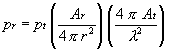
In our circuit, there are two antennas, the transmitting and the receiving antenna. The receiving antenna has a gain too. Multiplying we get



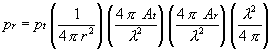
and this reduces to



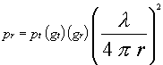
The distance and frequency-dependent term in the previous equation is the free-space path loss. Inverting it and taking the log generates the path loss equation on the previous page.

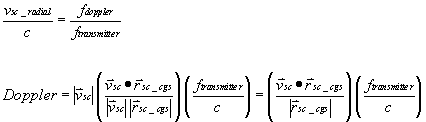
The Doppler frequency shift due to the spacecraft - CGS relative motion is derived first by determining the included angle between the spacecraft velocity vector and the spacecraft - CGS orientation vector.



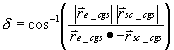
With this angle information, it is a simple thing to calculate the portion of that velocity vector that is parallel to the spacecraft - CGS vector and thus calculate the Doppler shift.



The s/c antenna generates two separate antenna beams, separated from on another by 6° and oriented at 40° and 46° from the s/c nadir. Due to geometry, these beams intersect the earth at approximate angles of 43.7° and 35.9° from the horizon. Neglecting atmospheric losses, there is less than a 0.005 dB potential variation in path loss due to orbit altitude variation.

2. Path Loss Variation Due to Atmospheric Effects

The Earth's atmosphere varies strongly in temperature, density and composition as a function of altitude. The primary classification of the regions of the atmosphere is according to the temperature gradient. Radio waves that travel from space to earth encounter four distinct regions. The first region is outer space itself; the next lower is the ionosphere, next lower is the stratosphere, and finally, where we all live and where all weather exists, the troposphere. Each layer has characteristics that affect the propagation of radio waves.



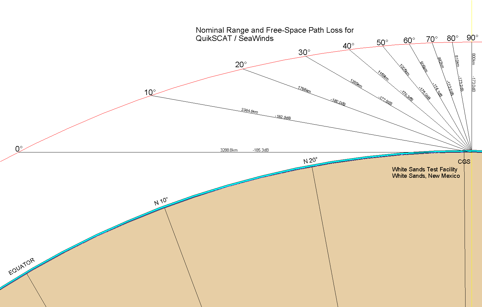
Figure -9 Path Loss and Range as a Function of Spacecraft Elevation

 

 

For our purposes, outer space provides lossless radio wave transmission. The ionosphere exists from 100 to 300 km above the ground. Here the pressure is low enough that the ultraviolet radiation that impinges on the earth from the sun causes a thin plasma to form as it separates electrons from atoms and molecules. These free electrons can affect a radio wave through effects such as Faraday rotation, reflection and absorption.

The stratosphere resides between about 15 km and 60 km. The atmosphere contained in this region is low density and very dry. However, the pressure is high enough that there is a very low content of charged particles. Due to these factors, radio wave propagation through the stratosphere is essentially lossless.

In this system the lowest part of the atmosphere (extended from the surface up to about 15 km) is called the troposphere, and it is bounded by the tropopause.

As described previously, the s/c generates two separate beams which intersect the earth at approximate angles of 43.7° and 35.9° from the horizon. This angle is neither grazing nor high-angle, but the radar signal must still pass through a substantial distance of atmosphere, not apparent from the vanishingly thin line that represents the top of the troposphere shown in Figure 3.9.

In Figure 3-10, the light blue region represents a 15 km atmospheric thickness (approximately the top of the troposphere, or the tropopause), while the dark blue zone underneath it represents the 4 km scale atmosphere used for modeling the effects due to oxygen.



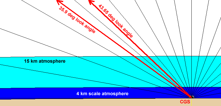
Figure -10 Path through the Atmosphere

 

Other factors include pointing error due to refraction of the radar beam as it passes from space into the atmosphere. At the relatively high elevation angles that are used for this station, the difference in apparent observed angle and geometric angle is very small and so this effect can be ignored [2].

3. Path Loss Variation due to Atmospheric Water, Oxygen and Other Airborne Substances

The atmosphere contains substances that can impact the transmission of radio signals passing through it. These materials include molecular oxygen, water, dust and other aerosols. At 14GHz, the primary impact on the radar transmitter signal is due to molecular oxygen and water as vapor and liquid.

1. Oxygen and Water Vapor

There is a local maximum in the atmospheric attenuation due to water vapor at approximately 22 GHz. At 13.4 GHz, this attenuation is not nearly so severe. For an earth-space link, total clear sky loss for a vertical path through the atmosphere is approximately 0.08 dB for water vapor and 0.04 dB for molecular oxygen [3]. In general, the paths along which the CGS will view the spacecraft are slant paths. A correction factor approximately equal to the cosecant of the viewing angle above the horizon should be applied.

2. Rain and Snow

Water as a liquid has dielectric and conductive properties that cause it to interact with electromagnetic radiation. As liquid, water can attenuate the received Ku-band signal through scattering, absorption and depolarization. In the instance of the CGS, depolarization is of little consequence since the receiving antenna is polarization-independent. The other two methods can strongly affect the performance of the CGS.

Generally, in the arid environment of the CGS, water in a liquid form occurs only as clouds, with rare rainfall. As clouds, not only does the path attenuation increase but the observed radiometric noise temperature goes up since the clouds reflect radiation coming from the warmer earth below. It may not be possible to adequately remove the effects of added attenuation due to clouds, but it may be via this increased noise temperature that we shall be able to successfully detect potentially suspect data.

If it decides to rain, though, attenuation can rise tremendously, with the potential for attenuation of 10 dB or more if a large rain cell is positioned directly in the path of the radio wave. Again, this can be detected in a number of ways, not only by radiometry but possibly by large increases in relative humidity and maybe even by physical rainfall recorded by the CGS weather station.

Finally water as solid, generally snow, occurs but is essentially transparent to the radar beam. The concern with snow (or ice) occurs if it finally turns to water. This is because there is the possibility that in the dry climate of southern New Mexico the ice or snow may actually sublime (go directly from solid to vapor phase). But, assuming that it does eventually turn to water, this can occur either in the air, if the snow passes through a warm air layer on its fall to earth, or once it has settled on to the radome. Once on the radome, there is a high probability that it will turn to water since the temperature of the air on the inside of the radome is much higher than that on the outside. Heat transfers, and snow melts. It is this melted snow as water that can very strongly absorb the microwave signal. It is also for this very reason that the primary surfaces of the radome are oriented vertically, so that collection and retention of liquid on the radome surface is very unlikely.

Liquid water can also condense onto the radome surface when dew point of the surface air is substantially higher than the inside temperature of the building. When this occurs, the radome could actually be cool enough to cause local condensate to appear. So long as the drops are very small and unconnected, this should not be a problem.

In all cases, the temperature of both the inner and outer surfaces of the radome will be closely monitored to reduce the probability that data taken has been corrupted by the potential formation of moisture.

5. CGS Design

Once the signal reaches the radome, it is in the domain of the CGS since, from this point on, the environment is completely controlled by the CGS. After passing through the radome, the antenna collects the signal and then the receiver's work begins. The receiver is the nexus of any overall system instability and so good receiver design is critical to reduce this. Reduction of the total count of components in the receiver chain is very important to reducing receiver instability. The use of high-quality, temperature-stable, low-noise components is fundamental also.

1. Radome

The radome is a cylindrical, "bullet-shaped" enclosure that fits over the antenna assembly and provides environmental protection to the antenna assembly (Figure 3-11). It also forms the seal for the top of the building and prevents outside environmental variation from strongly affecting the environment of the CGS. The radome is made of a impregnated honeycomb material that is sheathed in an inside and outside layer of fiberglass. It is designed to have very low loss at the frequency of operation through both the selection of the materials used and the adjustment of the honeycomb core thickness to set up a quarter-wave electrical thickness and thus reduce reflections.



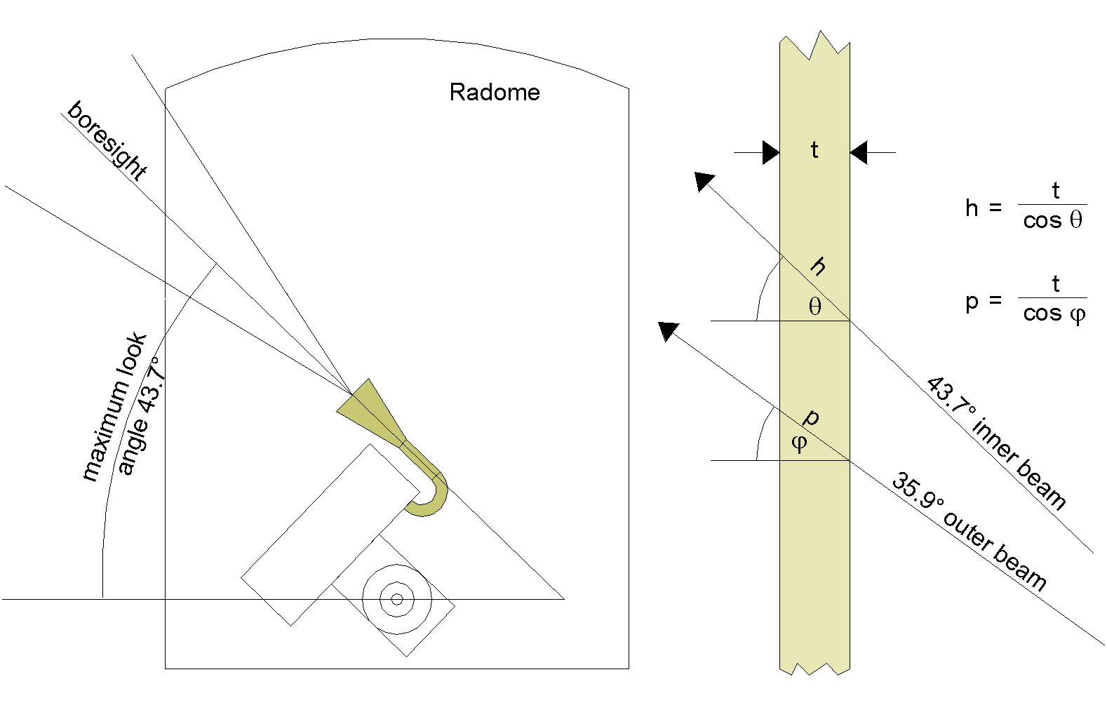
Figure -11 Radome / Observation Angle Profile

 

The use of the radome alleviates the particularly vexing problem of temperature control in maintaining a well-calibrated station. There are several approaches to insulating the antenna and receiver assembly from the environment. But most, in order to be effective, require putting some sort of barrier between the direct sun and the antenna. Rather than attempting to create a temperature-controlled enclosure that rides on the rotating pedestal assembly, it appeared easier to enclose the entire station including the antenna and thus isolate the equipment from the environment as much as practical.

The primary concern about impact to performance is the effect of the radome material on the incoming microwave signal. There will be a certain amount of absorption, reflection and refraction of the signal, and the radome surface will act as a collection surface for dust, water moisture, and other debris. It will also act as a diffuse scatterer to provide an alternate pathway for interfering signals either from other emitters or from multipath. Its finite loss will represent a small but measurable increase in the receiver noise temperature.

The use of a radome brings with it compromises. Without a radome, the view to the s/c is unimpeded, but some sort of mobile cover must be used to protect the station from inclement weather and other (avian) aerial bombardment. In addition, at some point before the observation cycle is to begin, the cover must be removed, radically changing the local environment of the antenna and structure and perhaps even of the receiver, due to solar insolation and exposure to the uncontrolled atmosphere. In addition, it becomes necessary, for an autonomous station, to determine what the outside weather is before opening the cover lest precipitation or airborne contaminants fall on the equipment. Another challenging problem for an autonomous station with a opening roof is one of personnel safety and equipment safety.

With a radome the effects of the outside environment can be tightly contained. With sufficient climate control inside the facility, it is nearly immaterial what the outside climate is (at least with respect to the performance and safety of the receiving station itself). With environmental stability comes station stability, which is critical for this application.

1. Losses Due to Radome Material and Construction

Materials used in radome construction are relatively low-loss at Ku-Band. In addition, a method known as "tuning" can be used to further reduce the effect of the radome on the desired signal. This method requires that the radome thickness be controlled to be approximately a 1/4 wavelength at the frequency of operation, minimizing reflection.

Some debate can be made regarding the choice of material for the radome [4]. A Styrofoam / Teflon skin structure is probably the ultimate for low-loss at this frequency, but it has a limited lifetime and in the harsh environment of the desert would quickly degrade. The more traditional choice of a fiberglass skin covering a Nomex honeycomb will have far better strength and longevity without sacrificing much more in the way to performance.

The construction of this radome is straightforward: first, the nominal path length through the finished radome is calculated. This requires knowledge of the geometry of the situation. In the case of the CGS, the s/c is observed only when the s/c radar beams intersect the CGS antenna. This occurs when the s/c is approximately 35.9° and 43.7° above horizontal. So the average look angle is about 39° . Once the physical shape of the radome is determined, the actual path length through the radome can be determined, allowing the final radome thickness to be precisely tailored to the incidence angle by cutting the honeycomb (99.9% air) to the appropriate thickness.

The surfaces through which the radome will observe the s/c must be kept as clean as practical in order that the measurement is relatively unaffected by dust, moisture and other debris. The most obvious choice for this surface is a vertical one, and the only way to have a vertical surface no matter the azimuth is to construct a vertically oriented cylindrical radome.

A cylindrical radome presents a smooth, vertical surface no matter where the s/c is in azimuth. This vertical surface is very resistant to collecting debris, and dew is unlike to form. Precipitation as rain runs off quickly and as snow is unlikely to stick to the surface. However, from a manufacturing point of view, the combination of relatively high look angles and the large extent of the receiving equipment means that the cylinder is large. Since it is desired to make the cylinder either seamless or with as few seams as possible, this constrains the size of the antenna and receiver structure that must be rotated within the radome.

Once an appropriate cylinder size is selected, the upper end must be capped. For this radome, we selected a stock paraboloid section (cheap and available since it is the basis of many antennas). The seam between the paraboloid section and the cylindrical section needs to be clean but the change in thickness and potentially dielectric constant doesn't impact the radome performance as the location of the seam is located approximately in the first null of the highest look angle.

2. Losses Due to Debris on Radome Surfaces

Material that can collect on the radome include water in liquid or solid form, dust, and organics. In the arid southwest, water in any form is infrequent. Wind-blown dust is more common. Organic matter (bird droppings, etc) is infrequent but possible.

In addition to increasing the transmission loss through the radome, the antenna noise temperature can increase due to this foreign material. It is important to control its deposition and to know when it is there.

Cameras externally mounted are used to observe the surface of the radome and estimate whether there is gross contamination that could impact the data observation. These images are cataloged with the received data but not examined unless the observed data is anomalous.

A weather station attached to the building records dew point, rainfall, and temperature. In addition, the temperatures of the outer and inner surfaces of the radome are measured and recorded. This way it can be determined whether there is a high probability of moisture condensation on the surface.

Minor dew where the individual drops remain unconnected to one another has a negligible impact on measurement [5]. Once the dew has become heavy enough that adjacent drops connect, the transmission losses can become formidable and the noise temperature can change drastically. So the uses of radome surface temperature and local dew point are critical here. In addition, since one of the daily observations will occur at dawn, this is a prime time for condensate formation.

Dust is generally non-conductive, very small in size, and has nearly zero effect on performance. Over time, though, the radome surface can collect enough dust (and other material) that there might be a measurable effect, so it is necessary to have a program of regular radome cleaning to remove any buildup.

3. Noise Temperature and Multipath Contribution Potential

System noise temperature should be as low as practical, but it is more important to make sure the system stability is high. Regular noise temperature measurements will not only provide a good estimate of system stability but also provide a good tool to calibrate the entire system including the radome and antenna, not just the receiver.

Multipath is a constant concern. The look angle of the antenna is relatively high above the horizon, but the CGS antenna beamwidth is wide and there are sidelobes that see the earth's surface along with structures local to the CGS. Multipath is the reception of unwanted signals radiated from the s/c transmitter reflected from local surfaces. These local surfaces can be many miles away. Detection of these unwanted reflections is nearly impossible due to the geometry of the observations and they can have a strong and very adverse influence on the desired measurement.

The potential effects of multipath must first be quantified and the geometry of the situation be understood. Physical control of multipath calls for the use of RF absorbing materials on immediate surfaces (rooftops, etc), and RF absorber fences employed to screen out the potential reflection points further away and out of the direct control of the CGS.

In the environment of the CGS, multipath should be a minor issue. The antenna main lobe is never closer to the horizon than 35.9° , the response continues to drop to better than -30dB at the horizon and the highest object nearby is a wooden telephone pole at about 18° . The first large, extended reflector is a range of mountains about 2 miles distant and as high as 11° above the horizon.

All of these potential reflectors are well off the main beam of the antenna. At elevation angles near the horizon, the antenna directivity will be off between 20-33 dB. With a single, perfectly positioned specular reflection, the impact on the desired measurement will be on the order of 0.02 dB. While this in itself is minor, the real world presents many potentially specular reflectors, lots of diffuse reflectors, and all these are in no particular phase relationship to one another. But they add to the ground clutter and can bias the measurement. So control of the potential interference from them is important.

This is where the RF absorber fence comes in. This fence surrounds the radome, and interferes with any direct path between the antenna horn and the points of reflection. The top edge of the fence is rounded to reduce the effects of edge diffraction, which is worse than diffraction off a cylinder.

As mentioned before, the radome can contribute adversely to the measured CGS noise temperature. In addition, it provides a very diffuse diffractor / reflector of stray RF energy that may illuminate the radome from undesired sources, like multipath.

Finally, it is possible that through long-term observation the effects due to multipath might be observed. Multipath will cause often-consistent and repeatable changes in the measurement as a function of look angle, and over time these changes might be able to be divined.

2. Antenna Subsystem

1. Horn Antenna and Waveguide Plumbing

The CGS antenna is a circular Potter [6] horn design, designed for strong sidelobe reduction. It was machined from a single piece of aluminum for rigidity and stability. The pattern for the operational antenna is depicted in Figure 3-12. The pattern is a hybrid of the pattern as measured on an antenna range from -90° to +90°, and a Bessel J1(x)/x pattern extends the skirts outside of ±90°, for field-strength modeling.

The CGS antenna incorporates a Kapton window assembly at the aperture that consists of two sheets of Kapton spaced by a quarter wavelength. This spacing helps to reduce the reflections from this surface and provides an excellent horn return loss (>40dB). At the other end of the antenna, a polarizer combiner allows a signal of any polarization to be received approximately equally. This combiner has been measured to be flat to better than 0.2dB independent of polarization, and the knowledge of the flatness is better than 0.02dB. All waveguide joints were lapped and securely fastened together, and all seams were sealed with silver epoxy. The entire assembly was then covered with absorber sheet to reduce sidelobe and backlobe interference. In the future, a more precise antenna calibration will be completed by the National Institute of Standards and Technology (NIST) at Boulder, Colorado, and will provide an absolute measurement of the antenna gain using a three-antenna measurement technique [7].



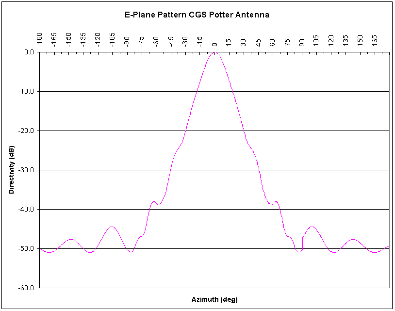
Figure -12 CGS Potter Horn Antenna Pattern, Measured + J1(x)/x (E-plane, azimuth)

 

2. Computer-Controlled Pedestal

A ground station designed and built for the NSCAT mission provided some of the raw components of the new CGS. The computer-controlled antenna pedestal was one of these items that could be reused. This pedestal allows movement through slightly more than 360° in azimuth and 90°+ in elevation. It employs servomotors that allow very fine position control on both axes, and 16-bit optical encoders to read back the position. It is capable of velocities exceeding 10° per second in any direction and has high position stability once at its final point. The station controller computer communicates with the pedestal controller interface via an RS232 line. Both command and position feedback are transmitted on this interface.

3. Interconnection to the Receiver

Simple interconnection to the receiver racks is achieved with flexible but electrically highly stable corrugated semi-rigid coaxial cables. These cables provide low loss, high dimensional stability, and are very rugged. They were tested for stability by moving the antenna while continuously observing the CGS noise source.

3. Receiver

The previous NSCAT ground station provided much of current receiver components and basic block diagram, from the receiver front-end and downconverters to the output of the second IF.

1. Frequency Plan

Simplicity is the key to a stable receiver. To that end, reducing the number of downconversions is an important tradeoff. Why is this a tradeoff? Fewer downconversions means that the RF and IF filter bandwidths required need to be more tightly controlled and very stable. But almost always this is a better choice than adding conversion stages and increasing the potential problems of more amplifiers, mixers and local oscillators. In addition, the more local oscillators and mixers used allow for more image rejection problems and more spurious energy generated locally that can affect the desired measurement.

The receiver design employed for the CGS is a superheterodyne that uses two downconversions. The first conversion is from the RF frequency of 13,402 MHz to the first intermediate frequency of 395MHz. The next conversion mixes the 395 MHz IF with a 360 MHz local oscillator to generate the final IF frequency of 35MHz. This second IF frequency is then digitized and signal-processed.

Receiver gain is controlled manually, and in general is preset to a single value for all measurements. This is practical since the target is well-known and characterized. If required, receiver gain can be increased in order to make very sensitive sky noise measurements.

2. Gain Diagram and Dynamic Range

Receiver gain is distributed throughout the system. At RF, medium gain with low noise is very important to overcome the noise figure contributions of the first conversion mixer. The first IF contains the bulk of the system gain. The second IF is a low-gain stage with the primary function to provide the final bandwidth filtering for presentation to the downstream digital converter. The receiver gain chart is contained within the System Link Budget in Figure 3-1. Receiver dynamic range is determined by the ratio of the weakest signal to the strongest signal. The CGS maximum received signal power is estimated to be approximately -68 dBm; the weakest signal is the noise floor itself at approximately -111 dBm. Thus, the receiver instantaneous dynamic range is 42 dB, which is not excessive.

4. From the Digitizer to the Customer

The data spooling out of the science analog-to-digital converter consists of 8-bit words sampled 41.9 million times per second. The information bandwidth contained in this high rate data stream is only about 1.5 MHz. It is therefore practical to immediately decimate this data stream to reduce its total volume.

The reason that sampling is done at such a high rate and IF frequency (35 MHz) is, as has been discussed earlier, to reduce the total number of analog conversions and components that the signal must travel through. Digital conversion of high frequency Ifs is very practical and relatively inexpensive and, once digitized, the information is safe from corrupting noise.

The data stream is decimated by a factor of 8 to provide the final data rate of 5.24 MB per second. This data is streamed into a 1 GB RAM memory that resides in the CGS Capture Controller. The sample window during a single point is exactly 10 seconds long, so over 52 MB of data are collected during this interval. There are a maximum of four points available during one pass, and the period between successive points ranges from 20 to 200 seconds. Since the efficiency in moving data out of the RAM buffer onto a hard disk is low, the RAM buffer is sized large enough so that pass data does not need to be removed from the RAM buffer until after the pass has concluded.

Once the pass is complete, the CGS digitizer moves the data in 100 ms blocks from its RAM buffer to its local hard drive to make a more permanent copy. There will end up being 100 files that contain the 10 seconds of pass data. (This file size was chosen so that no individual data file would be larger than 500 kB in size, drastically improving file manipulation time and speed.) Then, it signals the CGS station controller computer that the pass is completed and it then becomes the duty of the CGS controller to fetch the data from the capture controller and transfer that data to the 18 GB of hard drive storage on the server. Once on the server, data remains archived there for 7 days before it is expunged.

5. Data Product Generation

A software data analysis engine examines the archived data and begins analysis to extract details of the pass. The first data to be extracted is the rough timing pass data. The spacecraft transmitter pulse width and interpulse timing are well known a priori and a simple software filter goes through the data to find the individual pulses. Once these are discovered and tagged in time, further processing is done to extract precise timing, total relative energy in each pulse, timing jitter and amplitude stability during one pulse.

The next level of processing is in the frequency domain, with FFT analysis of the data files to extract both the spacecraft Doppler and the transmitter chirp. A dechirp template is used to find the best fit to the received data. Another estimate of per-pulse energy is made in the frequency domain by adding up all the power that appears in the few frequency bins that contain signal data. At this time, there are many more levels of data processing that are envisioned to eventually take place, but these will all be done in the future.

Once the processing has been finished, the results of the processing are saved as another file archive that is named with the day and time so that it can be correlated directly with the raw data.

Finished, archived data is stored on the CGS server computer. The server computer has an 18 GB storage capability using a pair of 9 GB hard drives. The files are named according to the date and time of capture, and files that contain weather observations and imagery for the same time period are also available. These files can be accessed by the user community via FTP.

6. Calibration

1. Noise Source

The CGS uses a calibrated, thermally controlled noise source as a primary signal level reference. The noise source is mounted in a aluminum enclosure that is insulated with blocks of rigid foam. A high precision thermal controller applies power to heaters attached to the sides of the noise source to keep the temperature of the noise source (as measured by a AD590 absolute temperature sensor) at 40 °C. The power to operate the noise source itself is controlled by an 8051 microcontroller, which receives serial data commands from the RS-232 interface in the data acquisition subsystem. The noise source also serves as a high quality load on the other port of the cross guide coupler when introducing a cal tone.

2. Frequency / Time Reference

A GPS / Frequency Reference unit provides a very stable 10 MHz reference signal with exceptionally low phase noise from a Temperature-Controlled Crystal Oscillator (TCXO), disciplined to GPS (Global Positioning System). This stable 10MHz output is provided as three identical signals at 1 V rms (+13 dBm into 50 ohms), and these are distributed within the CGS to provide very stable phase references. The first copy is used to phase-lock the 13,007 MHz receiver first local oscillator. The second copy is split at the receiver chassis and provides stable reference signals for the 360 MHz receiver second local oscillator and the 41.5 MHz digital sample clock oscillator. The last copy is used by the test synthesizer to generate highly stable and frequency-accurate microwave "calibration tones" that are then injected into the receiver front end.

This timing and frequency reference is based upon a free-running crystal oscillator which is of course subject to frequency drift. This is where the disciplining process becomes very important. The output of a ovenized VCXO is compared against the GPS signal. The difference in frequency is used to generate a correction signal which is applied to the voltage control port of the VCXO. The correction is primarily for aging, since the ovenizing makes the temperature sensitivity of the system quite low, providing temperature changes are less than about 8 degrees/hour (which they are, in our case). Even if the GPS signal is lost, the processor in the receiver will keep making periodic corrections, based on its calculations of the aging rate.

The correction signal is generated by a 16 bit DAC with a 0-5 volt swing. This swing moves the VCXO a total of 0.3 ppm (part per million), so a one LSB change in the DAC voltage is a change in output frequency of about 1 part in 10¹¹. The manufacturer claims that the time between updates is typically about 33000 seconds, after a 3-day stabilization period. Even if a step occurs during a capture, the magnitude of the step is so small that it will be well below the other noise sources in the system. Figure 3-8 shows the measured GPS/STALO performance over a 6-day period.



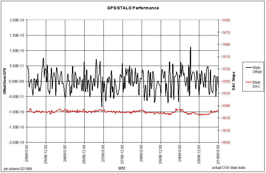
Figure -13 GPS/ STALO Performance over a 6-day Period

 

The primary factor degrading the frequency stability is the presence of Selective Availability on the GPS signal. The receiver attempts to track the random variations in the GPS clock and correct the VCXO for these changes. Therefore, once the system has stabilized, to achieve the most stable oscillator, the antenna should be disconnected so that the receiver does not try to track S/A. At this time it is not apparent that this will be necessary, but it is something that will be investigated as the CGS continues to operate.

3. Receiver Calibration

Without accurate amplitude and frequency calibration, the CGS would be of little or no value. Amplitude measurement accuracy has the highest importance, followed closely by frequency and timing.

1. Internal Calibration using the Noise Source

The internal noise source is a hot noise diode with about 14 dB (~7000 K) excess noise ratio (ENR). This noise source is maintained at 40.0° ± 0.1° in order to provide the most stable operating environment possible. A thermal controller using a microcontroller, precision platinum temperature sensors and conformal strip heaters allows very accurate and predictable temperature control.

The noise source can be switched into the receiver front end by reversing the polarity of the receiver front-end ferrite circulator switch [8]. When the noise source is not needed, the noise source DC power is shut off and the ferrite switch is set to the alternate position inserting over 30 dB of attenuation between the noise source and the receiver front end.

2. Radiometry

As a radiometer, the CGS has a number of calibration targets available with various utility.

1. Cold/Warm Loads

On the inner surface of the radome at 180° azimuth (due south) and 0° elevation (level to horizon) there is affixed a target made of pyramidal RF absorber material. This target provides a "warm" load at which the CGS antenna can aim and make radiometric measurements. There are temperature sensors embedded in the material so that an accurate temperature measurement can be made of the material and compared to the radiometric value.

There are plans afoot to include yet another absorber target but one that would also be cold, perhaps by running chilled water though a plate or even liquid nitrogen. Due to condensation issues, this has not been pursued any further at this time.

2. Sky

The sky presents a wonderful opportunity for extremely accurate calibration. It also allows end-to-end calibration of the entire CGS including antenna and radome. The galactic background at Ku-band is about 2.7 K temperature. Including the temperature contributions due to the radome, environment and sidelobe pickup, the CGS sees an antenna temperature of about 17 K. With the long integration times possible for the CGS, it will be practical to see variations in this noise temperature of less than 1 K even though the overall system temperature is about 250 K.

This ability to measure the sky will prove useful to accurately calibrate the radome characteristics. By performing "radome on - radome off" measurements [9], and scanning the cold night sky, a loss map of the radome may be possible. It may also be possible to see potential multipath sources.

3. Astronomical Objects

The sun represents a relatively bright (about 3dB NF), extended target that can be measured by the CGS receiver. There are future plans to incorporate the sun in receiver gain measurements, and potentially antenna pattern measurements.

The moon and all other astronomical objects pale (literally) in comparison to the sun in terms of power density per steradian. Due to the beamwidth of the CGS antenna, extra-solar system targets represent only a small fraction of the total energy received and so cannot be used profitably for calibration.

3. Other Spacecraft

There is the potential to make up of other spacecraft that are currently or planned to be up when the CGS is in operation. This will be pursued further in the future.

4. Remote Beacon Transmitter (RBT)

In August of 1998 it was suggested [10] that a Remote Beacon Transmitter (RBT) could be useful for at least checking the system function and perhaps more importantly, providing one solid and unmoving target to obtain some information about antenna boresight and pedestal alignment. In addition, the parts to manufacture such a RBT were available in the lab by cannibalizing the old ground station. Thus the RBT was born.



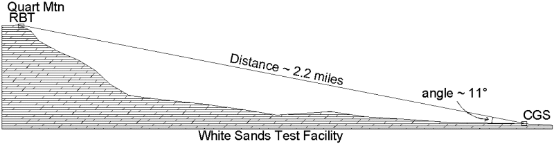
Figure -14 RBT Location with respect to CGS

 

The RBT is a solar-powered, radio-controlled device that sits atop a ridge about 4 km from the CGS (Figure 3-14). Upon command, it generates a monochromatic microwave pulse stream at 13,402.0 MHz and a pulse duration of 1.5 milliseconds. It uses a 0.5 m offset-feed paraboloid antenna with a beamwidth about 3° in diameter and switchable orthogonal linear polarizations to provide a signal that can be switched between horizontal and vertical polarization.

Control for the RBT is via standard pager receivers that have a contact closure option. The White Sands facility has its own pager network and thus calling a specific pager number activates the beacon. The RBT has a timeout circuit such that 10 minutes after it comes on it shuts off automatically.

The RBT is subject to temperature and weather extremes that affect its ability to produce an extremely accurate frequency and amplitude output. Care was taken in the design to use a temperature-compensated crystal oscillator that has a stability over the expected temperature range of better than 1 part per million (ppm), but even this is a large deviation (13.4 kHz) at the transmitter frequency. In order to reduce temperature and other environmental effects, a radome will be installed over the entire RBT protecting it from direct sunlight and rain while allowing sufficient air circulation to maintain an ambient temperature.

7. Mitigating System Gain Instability: Environmental Control

1. Temperature Control and Gain Control

With an analog system, temperature control is necessary for high amplitude stability. In the case of the ground station, temperature control is fundamental to the successful performance. Temperature control for the overall CGS is established with precise control of the environment inside the building housing the CGS. Dual 5-ton heat pumps keep a tight tolerance on the temperature excursions within the building. This temperature is monitored by the CGS control computer.

The pedestal-mounted equipment, thrust up into the radome, includes the antenna, the microwave receiver box and the antenna pedestal itself. The receiver box is a heavy steel and aluminum structure, with a large thermal mass and thus long thermal time constant, and is closed to prevent part cooling by convection. A fan inside the box distributes the air inside, keeping the overall air temperature inside the box very constant and distributing quickly the self-generated heat. The outside of the box is wrapped in a double layer of RF absorber foam, partially to reduce RF reflections and leakage, and partially to insulate the box from the outside environment.

The antenna and feed assembly is external to the receiver box, but is also swaddled in RF absorber material to provide insulation and equally importantly to reduce reflections and unwanted antenna surface currents that could affect sidelobe levels.

As evidence of the station's temperature stability, Figures 3-9 and 3-10 are plots of temperature from about 12 noon to 2:30pm on 02/09/1999 at the WSTF. Figure 3-10 shows the indoor and outdoor temperatures and Figure 3-11 shows the temperatures within the receiver chassis during the same time, showing the strong lack of sensitivity to the external environment.



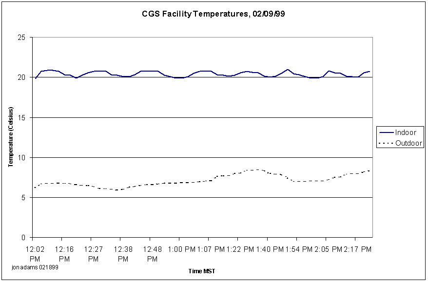
Figure -15 CGS Facility Temperatures



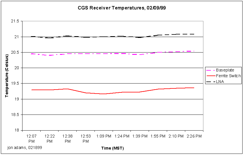
Figure -16 CGS Receiver Temperatures

 

2. Temperature Calibration and Characterization

Before installation at White Sands, the entire microwave receiver assembly was inserted into a thermal chamber and operated for a four-day period over a cycling temperature range. This was to simulate the effects of the diurnal temperature excursions at the CGS facility and to establish the basic temperature stability of the CGS receiver. Results of this testing indicated that over this period of time the receiver was very stable with respect to gain and phase and when returned to a given temperature would re-attain the original gain and phase.

 

4. Analyses

The following figures represent the output from the CGS Track Calculator software for a variety of passes as they would be observed from a CGS. For reasons of simplicity, it is assumed that the spacecraft is in a hypothetical equatorial orbit at 803 km altitude, and that the CGS is on the equator (for the zenith pass), and at latitudes increasingly distant from the equator for good mid pass, minimum pass, and missed pass.

1. Analysis of Good Pass (Zenith)

The figures 4-1 through 4-14 represent the output from the CGS Track Calculator software for a good (see ¶2.3.1) pass and specifically one where the spacecraft passes through the CGS zenith. The spacecraft illuminates the CGS twice with each the inner and outer beams.

Figure 4-1 is a plot of the spacecraft transmitter transmitted power density on the ground in the vicinity of the CGS. The plot represents a single good pass, traveling through CGS zenith, with the pass duration just under 1000 seconds. The points of interest in the plot are the four peaks, the two outer ones representing when the CGS is illuminated by the spacecraft outer beams (left hand is ascending, right hand is descending); the two inner peaks are the inner beam twice intercepting the CGS. The CGS receiver raw noise floor is about -111 dBm and the processed noise floor (after dechirp) is about 23 dB lower, at about -134 dBm. The model shows that there is plenty of power incident in the vicinity of the CGS in order to make observations, even when the spacecraft antenna is not aimed directly at the CGS. The coarseness of the four peaks is an artifact of the sampling done by the analysis software.

Figure 4-2 assumes that the CGS antenna is aimed at an elevation of 35.93°. The plot represents the gain of the antenna as a function of elevation. The plot to the right of center is a mirror-image, as if the antenna were moved to the opposing azimuth halfway through the pass.

Figure 4-3 overlays the CGS antenna gain (aimed at the 35.93° elevation) on the spacecraft ground power density profile and produces the power actually intercepted by the CGS antenna.

Figures 4-4 and 4-5 are the observed Doppler and range to the spacecraft. These are plotted to show that these are smooth functions and are amendable to linear interpolation over periods of 10 seconds, the nominal observation time.

Figure 4-6 zooms in on the plot of Figure 4-3, highlighting the peaks centered on the ascending outer and inner beam crossings. In the figure, there are 18 spacecraft antenna rotations visible and both the inner and outer beam peaks are recorded. Each tick on the plot represents one 1.5 ms transmitter pulse. The inner beam peak (right-hand) is depressed because the plot assumes that the antenna is fixed at the outer beam (35.93°) look angle.

Figure 4-7 zooms in further on the previous figure, highlighting the peaks that occur at the peak of the inner beam crossing. The center peak is when the CGS is fully illuminated by the spacecraft outer beam.

Figures 4-8, and 4-9 are the Doppler and path loss as observed by the CGS during the 10-second data capture window. Both Doppler and path loss are very smooth, essentially linear functions, the effects of which can be backed out of the captured data very easily. Figure 4-10 is the included angle between the spacecraft antenna boresight vector and the spacecraft - CGS direction.

Figures 4-11 and 4-12 are plots of the antenna directivities as a function of time. Of course, time is angle off boresight so it may be possible to estimate the antenna patterns based upon repeated measurements. Figure 4-11 is the spacecraft antenna directivity while 4-12 is the CGS antenna directivity (less the 3 dB for the loss in polarization). 4-12 is especially important as the CGS antenna is fixed in look angle during a single point, and the spacecraft drifts through the boresight. This indicates that if the spacecraft position can be later determined more accurately, it may be possible to extract most or all of the gain change due to position in the CGS antenna beam.

Figure 4-13 is a close-up of the single peak of the ascending outer beam. It shows more of the fine structure of the spacecraft antenna pattern, and each tick is a single transmitted pulse. There is a possibility that over repeated measurements that enough data points will be captured to paint a useful picture of the spacecraft antenna pattern.

 

 









 



















2. Analysis of Good Pass (Mid-Elevation)

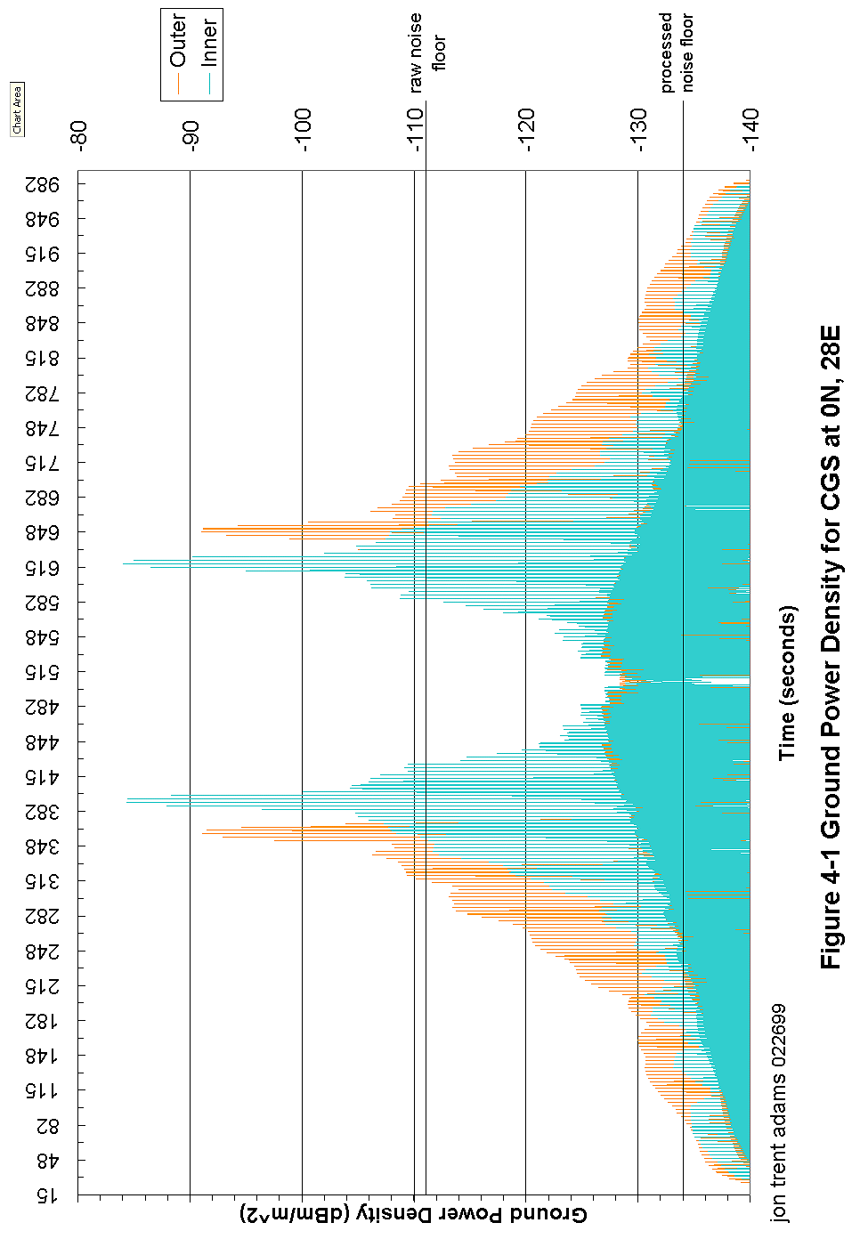
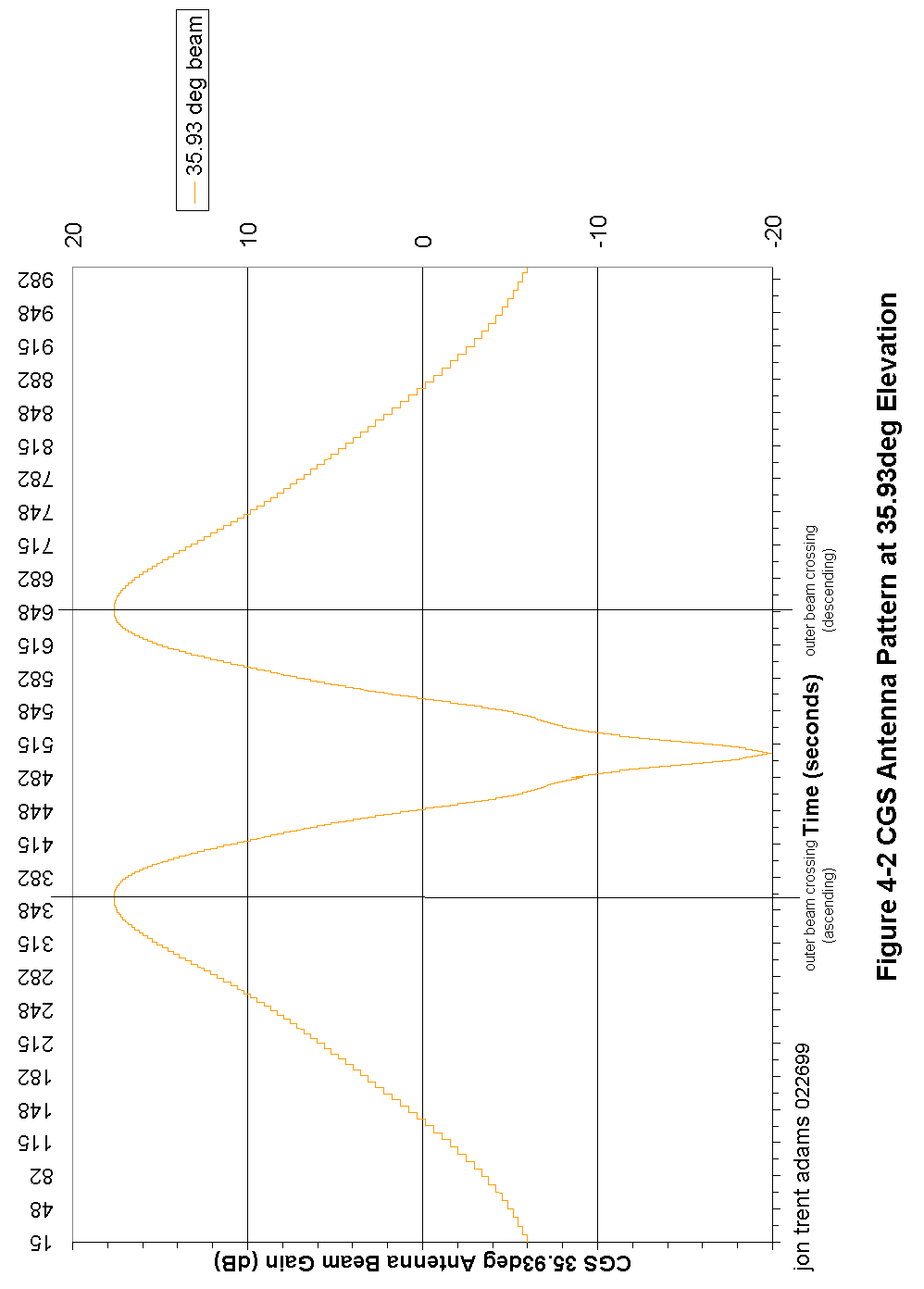
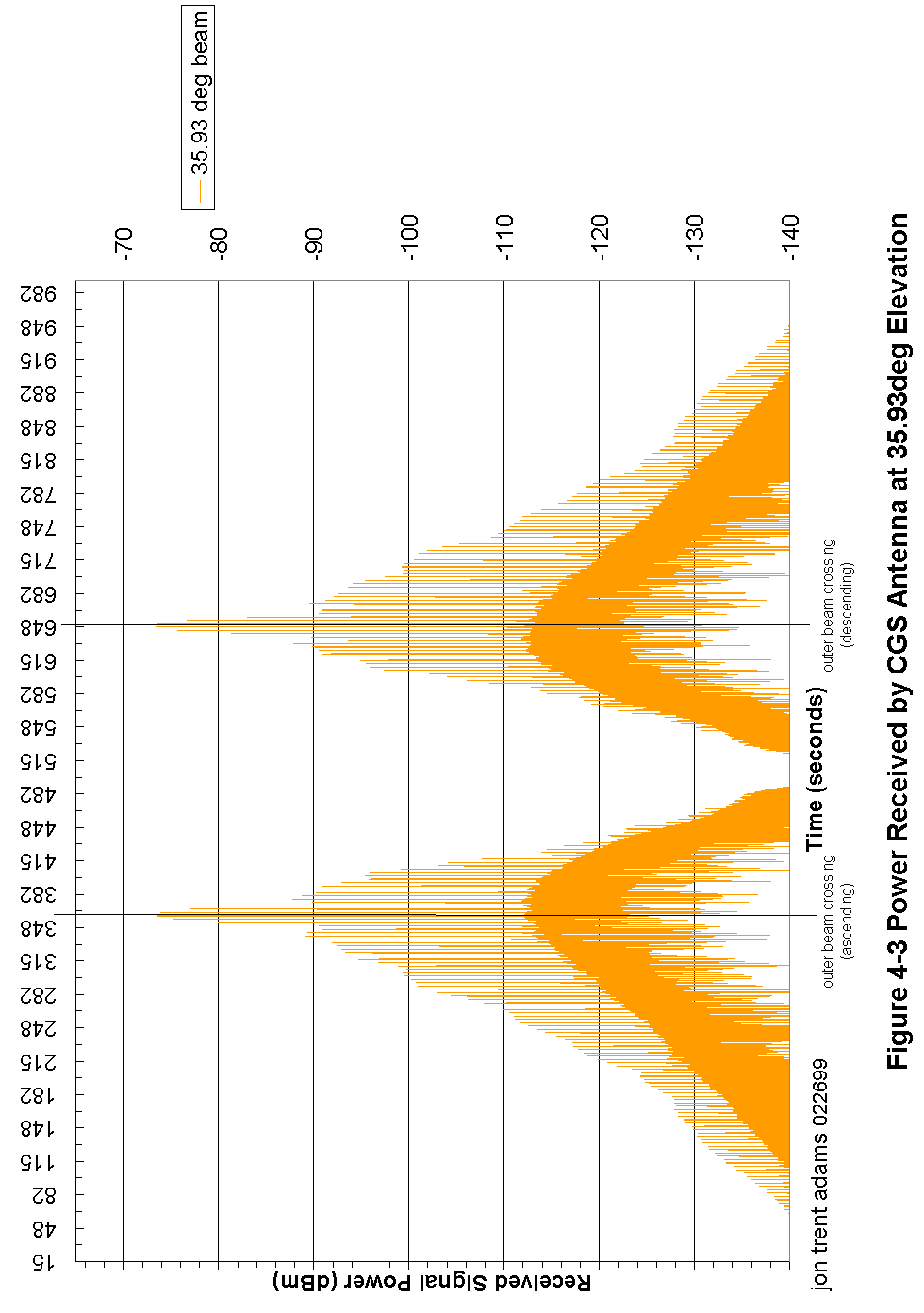
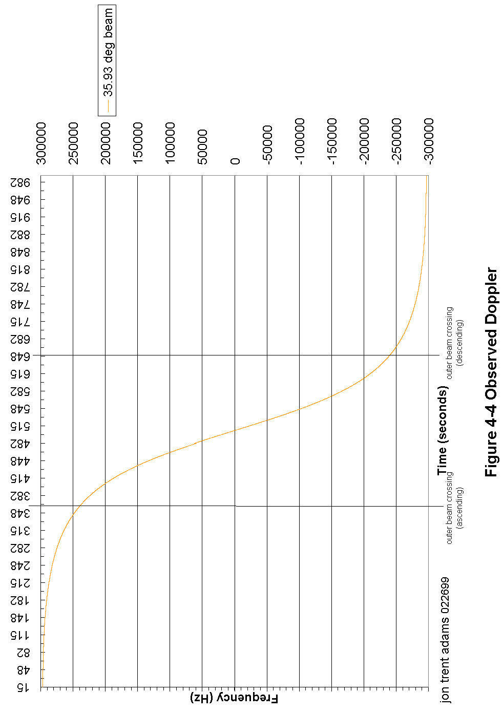
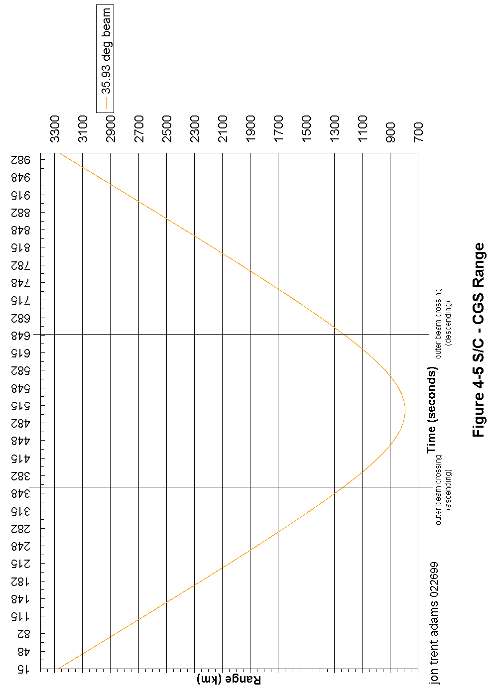
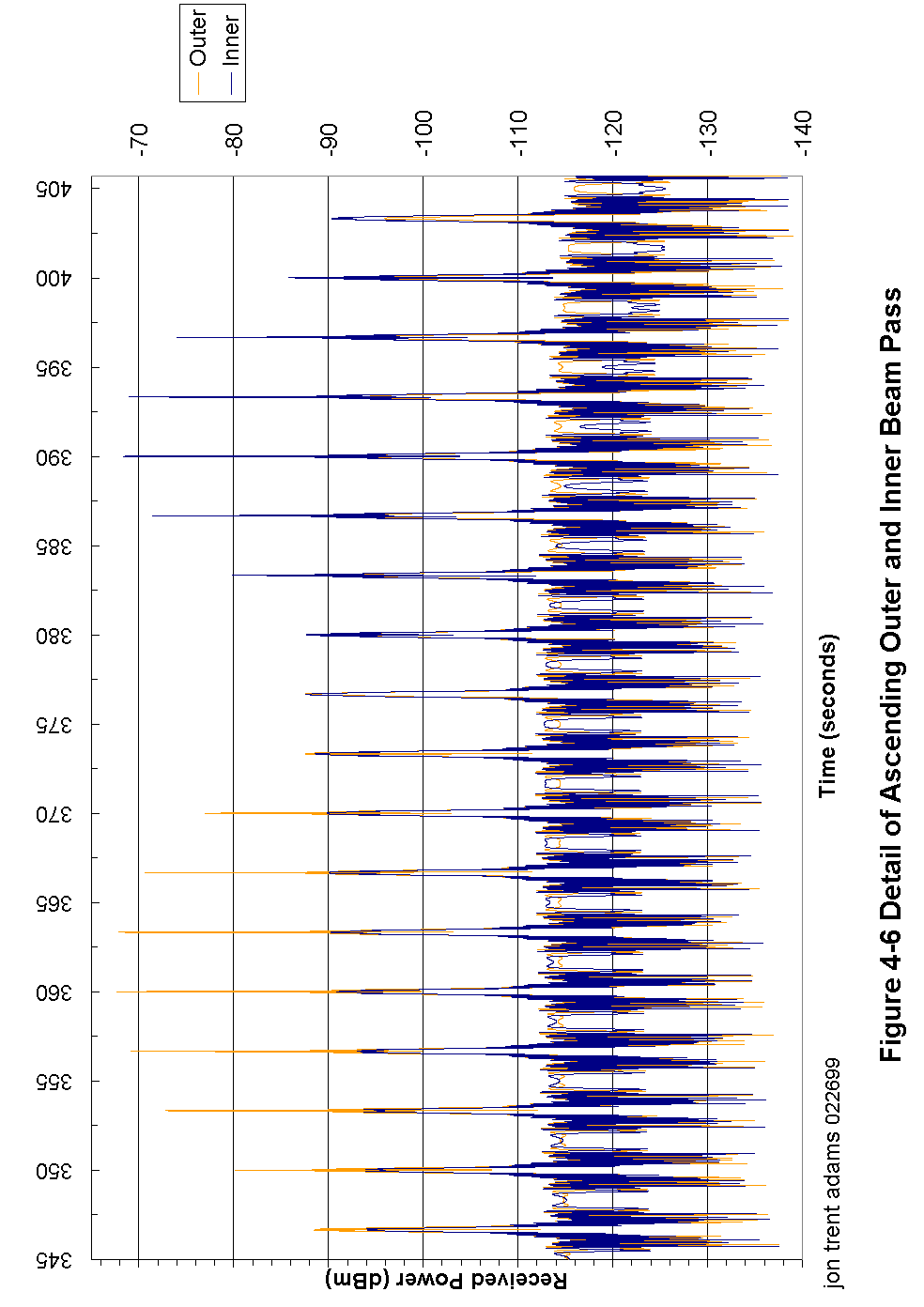
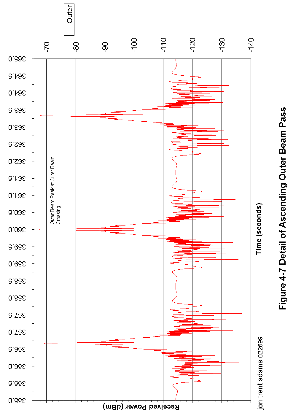
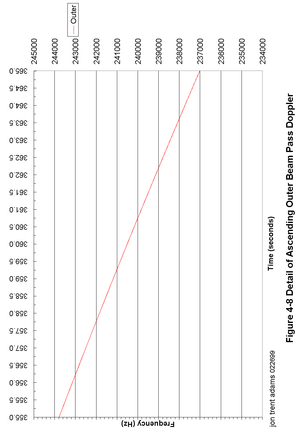
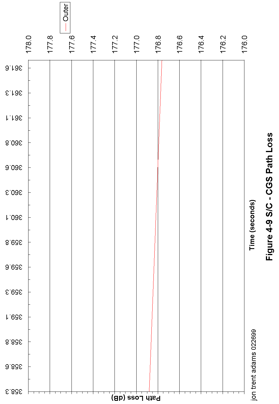
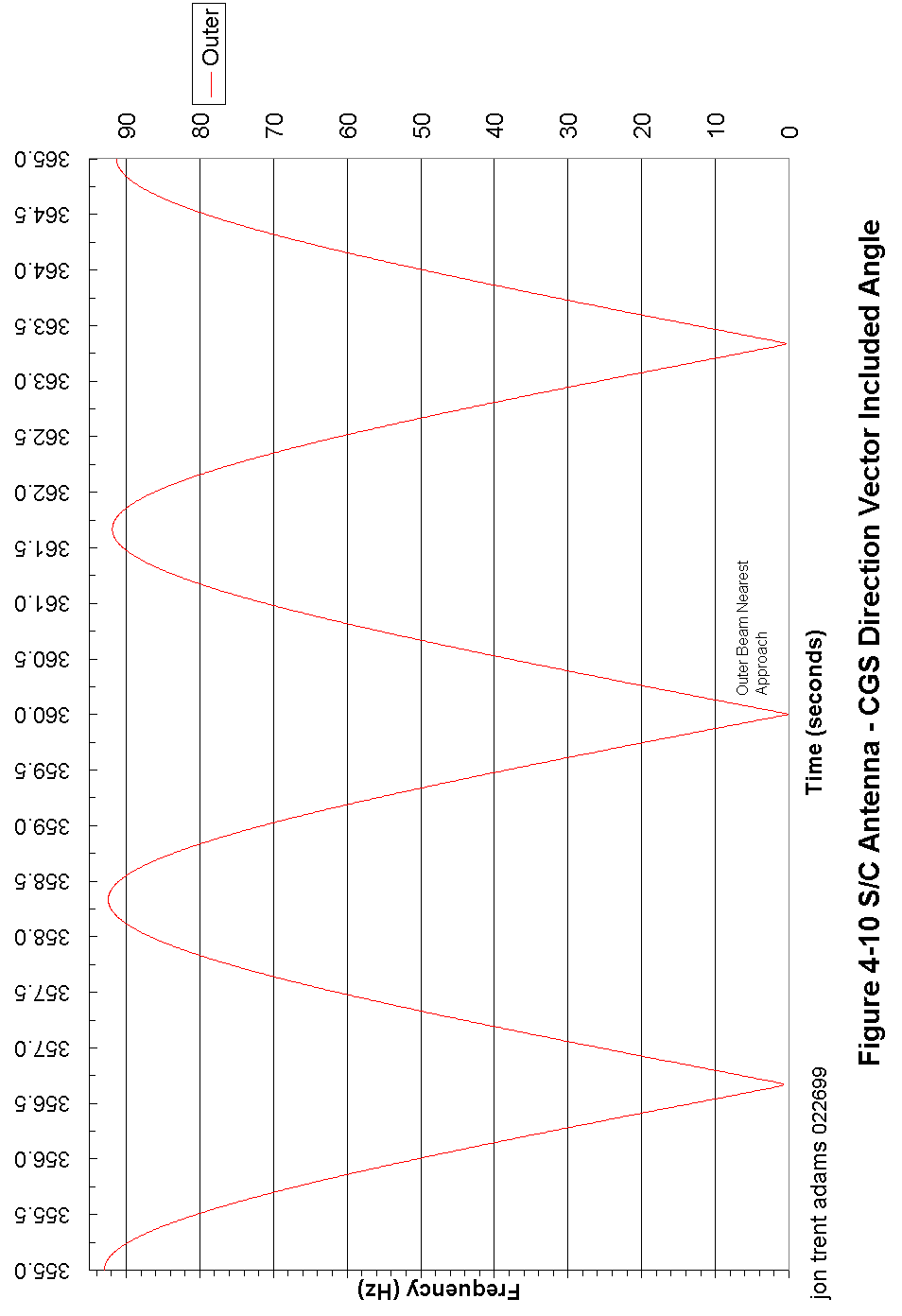
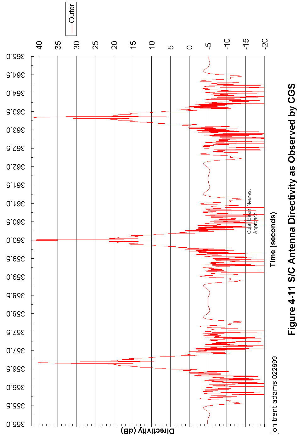
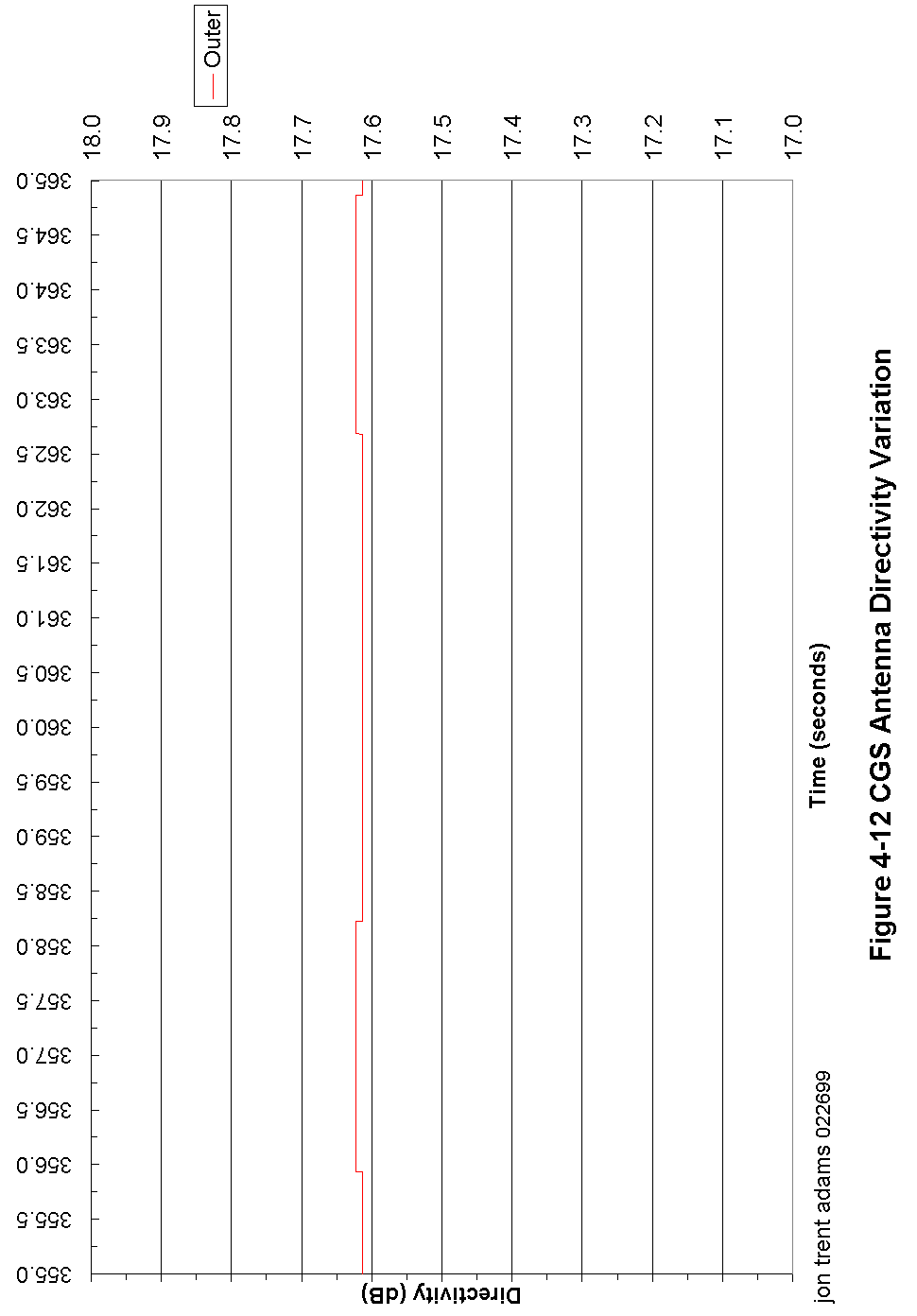
Figures 4-14 through 4-20 represent the output from the CGS Track Calculator software for a good (see ¶2.3.1) pass which is representative of a nominal pass where the spacecraft illuminates the CGS twice with each the inner and outer beams.

Figure 4-14 is the ground power density over the entire pass; 4-15 is the pass Doppler. 4-16 zooms in on the three pulses centered around the ascending node outer beam point and shows the ground power density during that time while Figure 4-17 shows the actual power collected by the CGS antenna while pointed at a nominal 35.93° angle. 4-18 and 4-19 represent the Doppler and CGS antenna gain variation during the same period. Figure 4-20 concentrates on the peak of the outer beam on the ascending point and shows the fine structure within.

 

 















3. Analysis of Minimum Pass

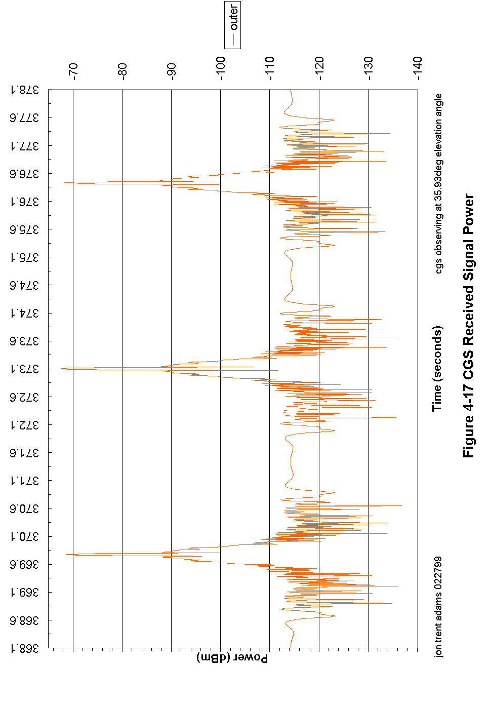
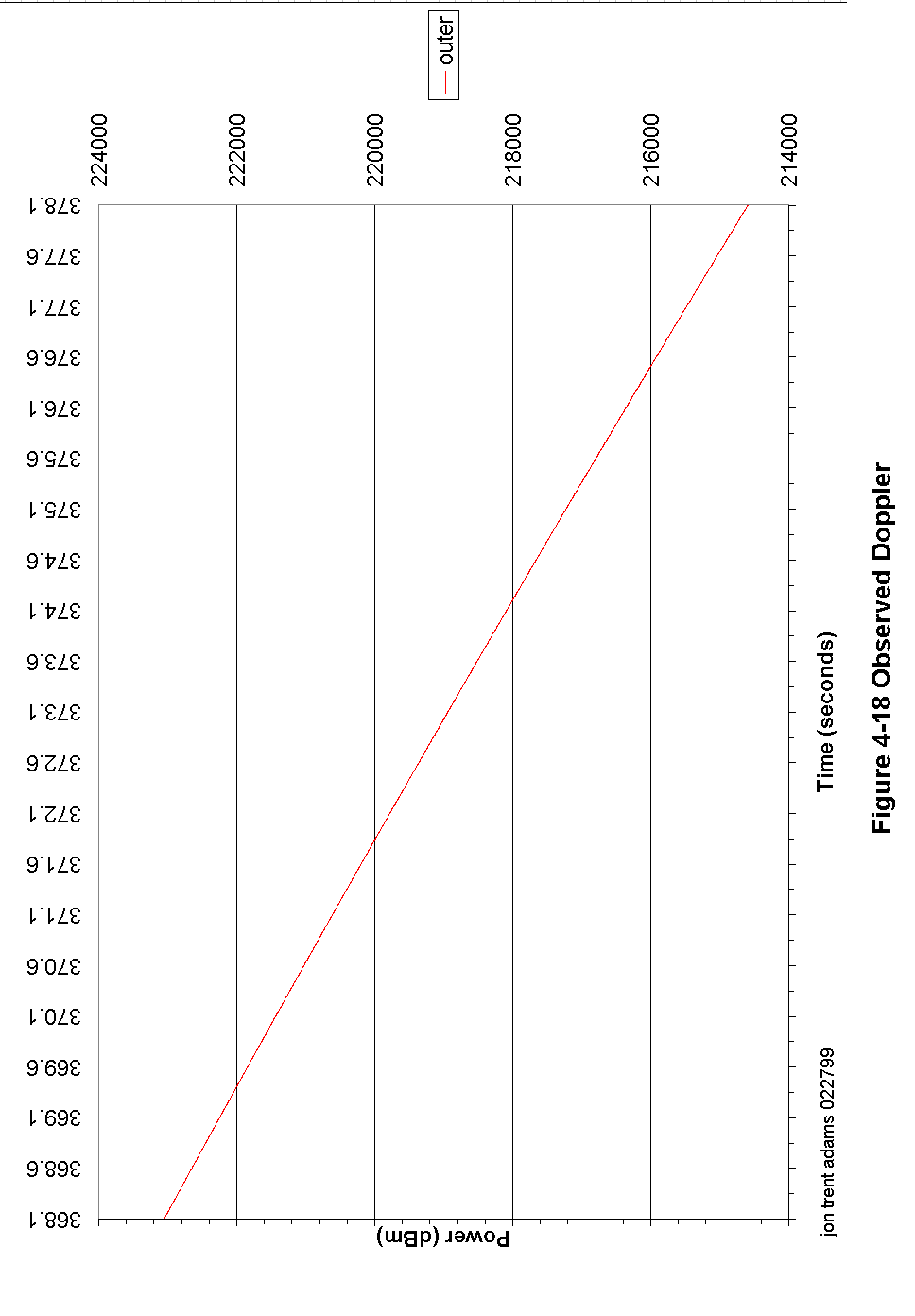
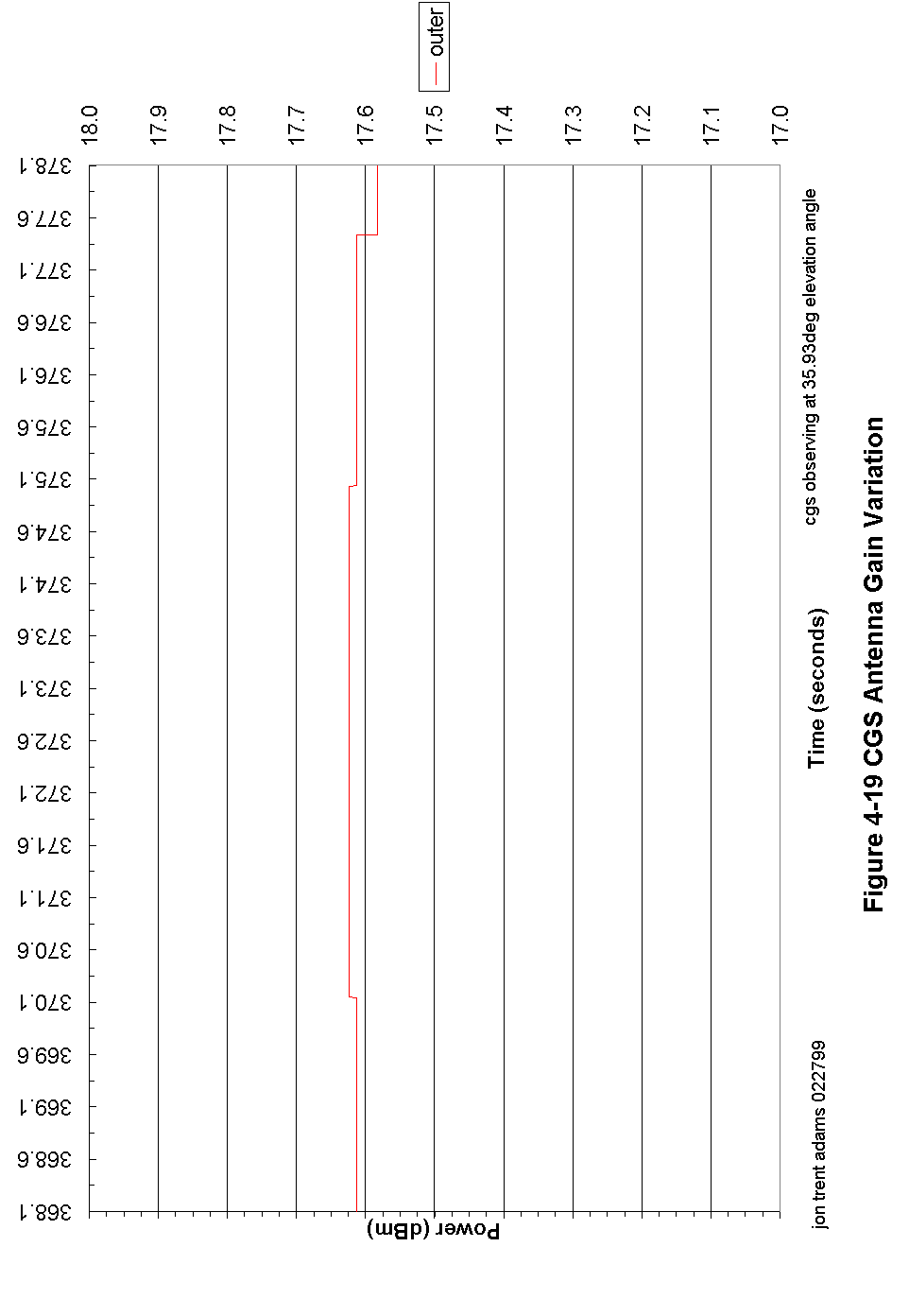
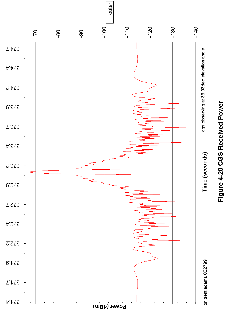
Figure 4-21 represents the output from the CGS Track Calculator software for a minimum (see ¶2.3.1) pass where the spacecraft rises high enough in the sky to illuminate the CGS twice with the outer beam only; or where the spacecraft rises high enough in the sky that the inner beam illuminates the CGS only once (and still twice with the outer beam). This figure indicates the ground power density during a minimal pass where the inner beam of the spacecraft never fully illuminates the CGS.

 



4. Analysis of Missed Pass

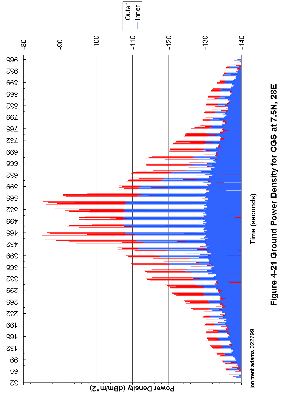
Figure 4-22 represents the output from the CGS Track Calculator software for a missed (see ¶2.3.1) pass. A missed pass is one in which the spacecraft does not rise high enough in the sky to illuminate the CGS with either beam. This means that any radiation that is received by the CGS is due only to spacecraft antenna sidelobes.

The most interesting thing about this figure is the fact that while the CGS is never illuminated by either the inner or outer spacecraft antenna main beams, there is plenty of ground power density available for the CGS to still make meaningful measurements of transmitter frequency and system timing, since many of the pulses are well above the processed noise floor of -134 dBm. And, if the CGS antenna is aimed toward the spacecraft's peak rise above the horizon, the 17 dB available gain from the CGS antenna will provide even better visibility of the spacecraft pass.

 



5. Conclusion
1. What Has Been Accomplished

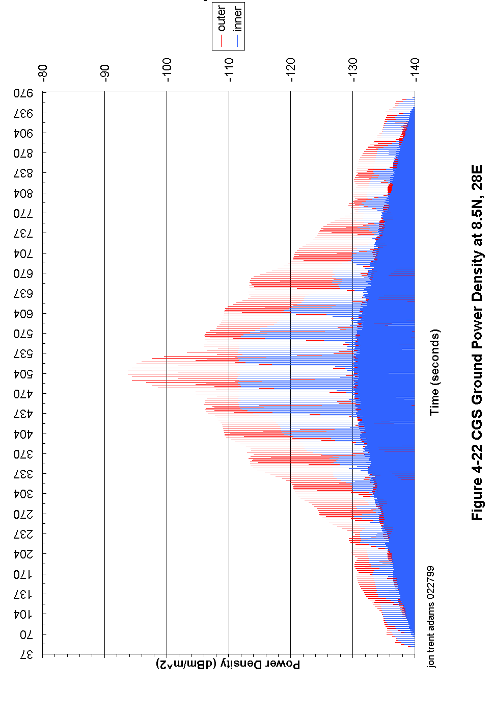
A Calibration Ground Station (CGS) has been built, tested and installed at White Sands Test Facility in New Mexico. Extensive calibration and testing of the CGS was performed to establish thermal and gain stability, and to properly characterize the CGS over a variety of operating conditions. From this testing and the analyses contained it appears that there is a high probability of success for this CGS to measure accurately important SeaWinds spacecraft instrument characteristics such as transmitter output power, pulse shape, pulse period, and Doppler offset.

There are significant challenges in doing this successfully due to the periodic rotation of the spacecraft antenna. The analyses indicate that the rotation of the spacecraft antenna may not be a significant problem, and in fact, may improve the ability of the CGS to measure the spacecraft antenna pattern.

2. Areas of Future Investigation

There remain additional tasks to be done, though, to further improve the quality of the data taken by the station. These include:

1. Characterization of the multipath environment. This effort has been begun with site mapping and empirical measurements by students from Brigham Young University. This data will be put into a multipath modeler and the results used to fine-tune the environment of the CGS. Large quantities of RF absorbing material are available and can be used to quiet the local environment.
2. More accurate measurement of the CGS antenna gain and directivity pattern. Both absolute accuracy and relative accuracy could be improved.
3. Extensive radiometric testing to characterize the radome and its loss contributions. The current loss estimate is based upon a single test sample and analysis of the geometry. This could be improved by a series of "radome on - radome off" measurements.
4. Perform a series of orbital analyses to determine the optimal orbit from the CGS point of view (i.e., maximum number of good passes).

1. Appendix

The software tool "CGS Track Calculator", was developed by the author for this thesis. CGS Track Calculator contains a orbit propagation kernel originally written by Dr. H. Scott Dunbar of the Jet Propulsion Laboratory. This kernel was written in FORTRAN, and re-coded by the author to run in Visual Basic 5. Figure 6-1 shows the user interface for "CGS Track Calculator".

All other software modules used in the generation of the raw data for this thesis were written by the author.

 

 



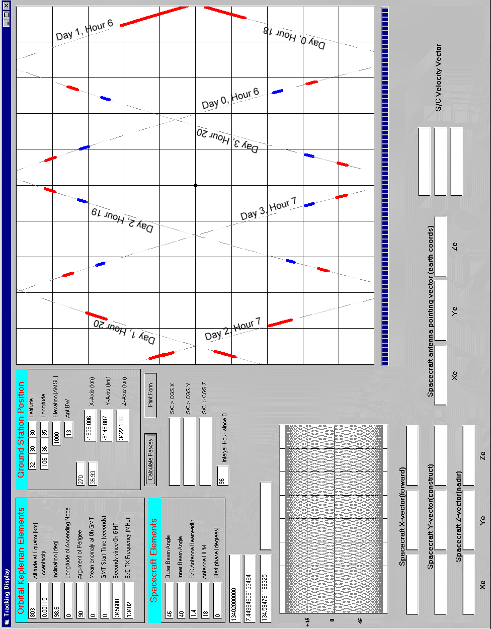
Figure 6-1 CGS Track Calculator User Interface

2. References
1. Specific References Called out in this Thesis

[1] Y. Rahmat-Samii, personal communication, Jet Propulsion Laboratory, February 1999

[2] F. Eaton, G. Nastrom and A. Hansen, "Middle atmosphere slant-path optical turbulence conditions derived from very high frequency radar observations", Soc. Photo-Optical Engr, Vol. 38, pp. 200-207, 1999.

[3] E. Jordan ed., "Reference Data For Engineers: Radio, Electronics, Computer and Communications ", Sams, Ch. 27, p. 29, Fig. 29, 1989

[4], [5] A. Tanner, personal communication, Jet Propulsion Laboratory, June 1998

[6] P.D. Potter, "A new horn antenna with suppressed sidelobes", Microwave J., Vol. VI, pp. 71-78, June 1963.

[7] W. Kummer and E. Gillespie, "Antenna measurements - 1978", Proc. IEEE Vol. 66, p. 483, 1978.

[8] C. T. Stelzreid and M. S. Reid, "Precision Power Measurement of Spacecraft CW Signal Level with Microwave Noise Standards", IEEE Trans. Instrumentation and Measurement Vol IM-15, p.318, 1966.

[9] B. L. Seidel and C. T. Stelzreid, "A Radiometric Method for Measuring the Insertion Loss of Radome Materials", IEEE Trans. MTT Vol. MTT-46, p.625, 1968.

[10] J. Lux, personal communication, Jet Propulsion Laboratory, August 1998

2. General References

D. Duan and Y. Rahmat-Samii, "Novel Coordinate System and Rotation Transformations for Antenna Applications", Electromagnetics, 15:17-40, 1995

K. Davies, "Ionospheric Radio Waves", Blaisdell Publishing, 1969

M.P.M. Hall, "Effects of the Troposphere on Radio Communication", Institution of Electrical Engineers, 1979.

N. Skou, "Microwave Radiometer Systems: Design and Analysis", Artech House, 1989

C. Balanis, "Advanced Engineering Electromagnetics", Wiley, 1989

R. Elliott, "Antenna Design and Theory", Prentiss-Hall, 1989

"Transmission Systems for Communications", Bell Laboratories, 5^th ed., 1982

C. Elachi, "Introduction to the Physics and Techniques of Remote Sensing", Wiley, 1987

J. Kraus, "Antennas", McGraw-Hill, 1950

F. Chen, "Introduction to Plasma Physics", Plenum, 1977

E. Jordan, ed., "Reference Data for Engineers: Radio, Electronics, Computer and Communications", 7^th edition, 1989

D. C. Cox and H. Arnold, "Results from the 19- and 28-GHz COMSTAR satellite propagation experiments at Crawford Hill", Proc. IEEE Vol. 70, p. 458, 1982.

D.C. Cox, "Design of the Bell Laboratories 9 and 28 GHz COMSTAR beacon propagation experiment", IEEE ICC, Minneapolis, MN, pp. 27E1-27E5, June 17-19, 1974.